Input data determination for assessment of flutter resistance of small aircraft

The category of small aircraft up to 600 kg maximum takeoff weight has developed significantly in recent years, particularly in Europe. Previously, ultralight aircraft up to 450 kg did not require an aeroelastic assessment (AE), except for unconventional designs or aircraft with cruise speeds above 200 km/h. However, these assessments are now mandatory for UL2, CS-VLA and CS-LSA type certificates. This requirement is mainly due to the rapid increase in airspeed of aircraft in this category, driven by new design approaches, the use of composite materials and increasing engine power (up to 150 hp).

Aeroelastic analysis deals with the interaction of three kinds of forces, i.e. elastic, inertial and aerodynamic forces. This interaction leads to a few aeroelastic phenomena under certain conditions, flutter being one of the most dangerous. The methods used to analyze the resistance of an aircraft to flutter and other aeroelastic phenomena has been developed and established progressively during the development of aviation since its beginning. The first methods were limited to very approximate solutions where the aerodynamic action was considered quasi-stationary, e.g. the use of Galerkin solutions (Duncan, 1937) of the differential equations of motion describing the aeroelastic system at its stability limit as described in Fung (1969). A more accurate determination of the dynamic aeroelastic stability limit required the study and establishment of methods for determining the aerodynamic forces and moments on the oscillating airfoils and wings. These efforts led to the establishment of more accurate methods for flutter calculation. One of the first methods in practical use is referred to as the “v-g” method (Smilg and Wasserman, 1942). This method works with the concept of structural damping, which allowed the graphical representation of the flutter solution in a diagram of the dependence of (artificial) damping on airspeed.

With the development of computer technology and numerical methods for solving structural and aeroelastic problems, methods for modal aeroelastic analysis such as the k method and the p-k method have been developed (Hassig, 1971). These methods are still widely used today and are also implemented in computational tools. Over time, the standard aeroelastic tool for strength analysis has become the product MSC.Nastran, which of course includes aeroelastic analysis with evaluation in the form of “v-g” diagrams, both for the subsonic and supersonic regime.

In general, it could be assumed that there are no complications in this area and that classical methods will guarantee a reliable calculation of the critical flutter rate. However, it turns out that the main obstacle in the analyses is the lack of the main stiffness characteristics to reliably determine the required critical velocities. Especially for composite aircraft, the scatter of material properties is significant. A number of researchers have addressed this issue by approaching the problem by introducing uncertainties (aerodynamic, mass and stiffness) into the equations describing flutter (Beran and Stanford, 2013; Leijonhufvud and Karlsson, 2011; Lokatt, 2017).

Based on the results of aeroelastic analyses of a number of small sport aircraft, this paper presents the results and experience of the Institute of Aerospace Engineering of the Brno University of Technology in evaluating the effect of input data scatter in terms of stiffness on the resulting determination of the critical flutter speed.

The method described in this paper is not limited to small aircraft but is also widely applied across various other aircraft categories. It has been successfully used for unmanned aerial vehicles (Bras et al., 2022; Chin et al., 2020), highly flexible high-altitude long-endurance (HALE) aircraft (Sharqi and Cesnik, 2024), general aviation aircraft (Spivey et al., 2022), gliders (Ozkok and Weltin, 2009) and large commercial aircraft (Göge et al., 2007). These applications highlight the broad relevance of the approach, demonstrating its adaptability in addressing aeroelastic challenges across different aircraft types and configurations.

The regulations governing the design of the aircraft category addressed in this paper are CS-VLA and CS-LSA. The requirements for certification of resistance to flutter and other aeroelastic phenomena are generally based on CS-23.

Under CS-VLA, which applies to very light airplanes with a maximum takeoff mass of up to 750 kg, it is necessary to demonstrate that the airplane is free from flutter, control reversal and divergence under all operating conditions within the V-n envelope and at all speeds up to the speed specified for the selected certification method. These methods include the application of a rational analysis, which must show that aeroelastic phenomena will not occur at all speeds up to 1,2v_D, and aeroelastic flight tests, which must meet the prescribed criteria. In addition, tolerances must be established for quantities affecting flutter such as velocities, damping, mass balance and control system stiffness. If the v_D speed is higher than 259 km/h, the natural frequencies of the main structural units must also be determined by vibration tests or other approved methods.

The CS-LSA regulation, which applies to light sport airplanes with a maximum takeoff mass of 650 kg, requires ground vibration tests followed by analysis of vibration modes and frequencies and potential flutter events for airplanes with a v_NE exceeding 200 km/h.

Both regulations allow the demonstration of aeroelastic performance of specified conventional airplanes by meeting the stiffness and mass balance criteria specified in Airframe and Equipment Engineering Report No 45. However, this option is only applicable to conventional airplanes that meet the design criteria specified in the regulations.

This section outlines the procedure for experimentally obtaining the dynamic structural properties of the aircraft. It covers the general test requirements, including aircraft suspension, sensor and exciter placement and data evaluation. The final part of the section provides a summary of the results from ground vibration tests performed on several aircraft at the Institute of Aerospace Engineering, Brno University of Technology.

The basis for the analysis of aircraft resistance to flutter and other aeroelastic phenomena is the identification of the dynamic behavior of the aircraft structure, including natural frequencies, mode shapes and damping ratios. This analysis is typically performed through ground vibration testing of the airplane in critical configurations, with emphasis on mass configuration – light and heavy and the control system state – free and fixed control stick and pedals.

The ground vibration test (GVT) is conducted in accordance with Advisory Circular AC23-629-1b (US Federal Aviation Administration (FAA), 2004), which not only covers the GVT but also provides general information for flutter proofing.

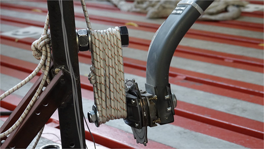
During the measurement, the aircraft is suspended by a bungee-based soft support with a natural frequency less than half the lowest natural frequency of the aircraft structure. The aircraft is normally suspended by its landing gear legs as it is shown in Figure 1. This suspension provides free-free conditions similar to those experienced by the aircraft in flight. During the GVT of each mass configuration, the frequency of bungee support is verified.

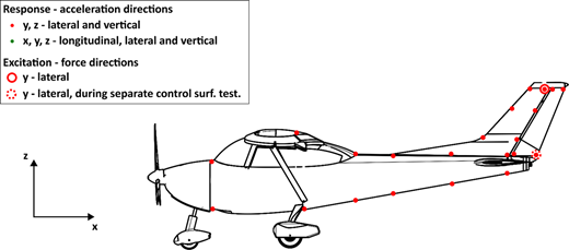
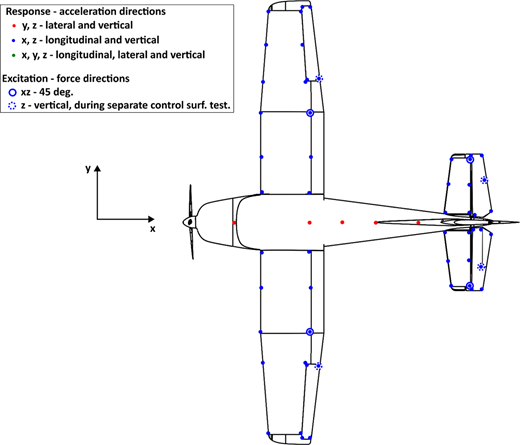
The excitation of vibrations during the GVT is done by electrodynamic shakers located in appropriate positions. In our case, it is usually at the wings tip, elevator tips and rudder tip locations. During the identification of control surface dynamic properties, the shakers excitation is brought to the surfaces at their trailing edge. The force is transmitted to the structure via a stinger rod, eliminating lateral inputs. The excitation force is measured by a force transducer positioned between the stinger rod and the aircraft structure. An auxiliary part was attached to the sensor.

The response is measured using the accelerometers located at the aircraft in such manner that it is possible to identify the most important mode shape of the airframe vibrations. The typical layout of responses and excitation location is illustrated in Figures 2 and 3.

Vibrations are excited using a stepped-sine signal within the frequency range of 5–105 Hz, with a frequency step size of 0.25 Hz and a settling time of 10 periods per step. During the initial run, the exciters operate in phase. In the second run, the phase of one exciter is shifted by 180 degrees, creating an out-of-phase excitation pattern.

Due to the limited number of sensors available, the roving response method is used. The measurement process is segmented into multiple stages, with accelerometers being relocated after each stage to acquire a complete response profile.

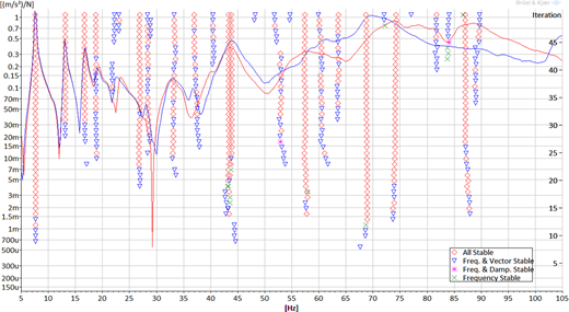
The software used for preprocessing, measurement and postprocessing tasks is BK Connect (Brüel and Kjær, 2019). Temporal data from the accelerometers and force transducers is processed in real time using Fast Fourier Transformation (FFT) to compute the frequency response function. This function is subsequently analyzed using specific criteria, typically the Rational Fraction Polynomial-Z (RFP-Z) method, resulting in the generation of a stabilization diagram (see Figure 4 for an example). From this diagram, the natural frequencies, damping ratios and corresponding mode shapes of the aircraft structure are extracted and identified.

Flutter resistance and other aeroelastic phenomena have been successfully tested at the Institute of Aerospace Engineering for a total of seven aircraft, each with a maximum takeoff weight of 600 kg. Three of the aircraft had airframes made from aluminum alloy, whereas the remaining were constructed from composite materials.

The outcome of the ground resonance test for each aircraft includes the determination of natural frequencies, vibration modes and the damping ratio of the airframe structure and its control surfaces. The natural frequencies for selected vibration modes of the airframes are listed in Table 1, where the aircraft are categorized by type of material and wing configuration.

The identified natural frequencies of control surfaces rotation for the same aircraft are listed in Table 2 for the free and fixed control stick and pedals.

This section provides a detailed overview of the preparation of the elastic and mass finite element (FE) models, the validation of the computational modal analysis against results of the ground vibration test and the development of the aeroelastic model. The concluding part presents the results of the flutter analysis. In addition, a discussion on the balancing of control surfaces is included, highlighting its critical role in preventing flutter below the 1.2v_D limit.

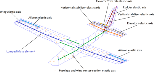
The primary input for aeroelastic analysis is the elastic model of the complete aircraft. Typically, this model is built using 1D BEAM elements with properties defined by a PBEAM card to represent the entire structure, see Table 3. These elements are positioned along the elastic axes of the fixed components, such as the wing, stabilizer, fin and fuselage and along the elastic axes of the control surfaces, such as the ailerons, elevators, rudder and trim tabs.

The elastic behavior of these elements is characterized by four key properties: the cross-sectional area A, the two perpendicular second moments of the area I1 (usually the bending of the wing) and I2 (the in-plane bending of the wing) and the torsional constant J and the material properties. These parameters are derived from the geometry and material properties of the respective structural sections. The exact determination of these properties is complex and often subject to considerable uncertainty. Therefore, it is not possible to define the exact position of the elastic axis, the cross-sectional area, the bending stiffness in two directions and the torsional stiffness for each cross section.

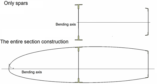
The traditional division of aircraft structures into beam elements for bending and torsion boxes for torsional loads is not sufficient to accurately determine stiffness properties. The entire structure contributes to both bending and torsional stiffness, a phenomenon that becomes even more significant when composites are used. Computer-aided design (CAD) systems can assist in the determination of bending moments of inertia by analyzing the cross-sectional geometry of the structure, see Figure 5. These systems can provide more accurate calculations for both bending and torsional stiffness, considering the contributions of the entire structural configuration.

The difference between the second moments of inertia I1 (wing bending) calculated by dividing the structure into bending resistant components and those calculated for the entire structure as a whole is considerable as it is shown in example in the Table 4:

However, while CAD systems can accurately determine bending stiffness, they cannot calculate torsional stiffness. This requires the use of analytical methods.

The formula for torsional constant J for torsion box (single cell) is:

where A is area of cell, t_i is thickness of skin or spar web and s_i is length of skin or spar web.

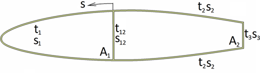
This equation is valid for a single cell. However, many aircraft structures consist of several closed sections. A simplified formula can also be derived for a double cell structure, see Figure 6:

where:

where A_i is area of cell, t_i is thickness of skin or spar web and s_i is length of skin or spar web. The coefficient a_ij is defined as a contour integral along the neutral line of the thin wall between areas i and j. The indices i and j take values 0, 1 and 2, representing the area outside the wingbox, inside the first wingbox cell and inside the second wingbox cell, respectively.

A comparison of the resulting second moments of inertia for single cell and double cell configurations is shown in the Table 5.

The mass model for aeroelastic analysis of small aircraft is developed based on a detailed mass analysis, the geometric model and the actual weights of individual aircraft components provided by the manufacturer. For most components, both the precise weight and the center of gravity can be determined in this manner. In aeroelastic analysis, this data is incorporated into the FE mass model, typically using 0D CONM2 elements, with input data shown in Table 6, which allow the specification of both mass and moments of inertia. However, accurately determining the moments of inertia for individual components is often complex.

To address this challenge, the mass FE model can approximate moments of inertia by dividing the individual components into a greater number of CONM elements. This method effectively distributes the mass and replaces the need for directly inputting moments of inertia. The finite element model (FEM) can then manage both the mass of the components and the position of their centers of gravity, such as for the wing or control surfaces like the rudder. Figure 7 illustrates a typical FE model, where 1D elements represent elastic axes and 0D elements represent mass distribution.

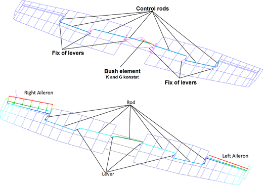
The FE model of the control link in the flexible FE model consists of the rudders themselves and the controls. The rudders themselves are replaced in the FE model by beams in the elastic axis of the rudder. The connection of the individual rudders to the support structure is then made by rigid body elements (RBEs) where the degrees of freedom are determined to match those of the true rudder. The actual rudder path, i.e. the rods and levers, is again modeled using 1D elements. The elevator and rudder control paths can be largely replaced by CBUSH spring elements whose properties are defined by PBUSH cards Table 7. Thus, it is not necessary to model the entire steering travel, most of the travel can be replaced by a spring element with suitable stiffness and damping. This elastic element will then provide the correct path stiffness and rudder oscillation. However, this approach cannot be used for aileron steering linkage where the connection between the left and right ailerons must be maintained as shown in Figure 8. The spring can be introduced into the linkage after the connection between the left and right ailerons has been established.

The stiffness of the elements used is then determined for both locked and free steering cases. These values shall be calibrated so that the oscillation of the control surfaces (their rotation about the hinge points) corresponds to the results of the ground resonance test.

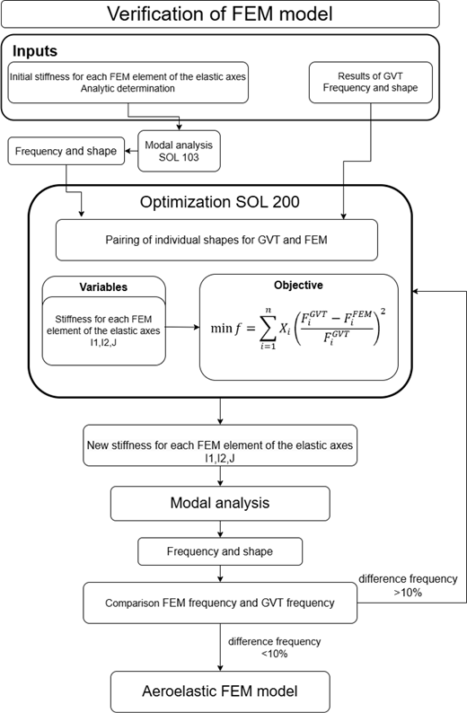
From the previous chapters, it is evident that the initial FE model for assessing aeroelastic resistance is significantly inaccurate and requires comparison and calibration against the results of the ground vibration test. This can be achieved through modal analysis. The outcomes of these analyses include the natural frequencies and mode shapes of the FE model. These mode shapes and frequencies are then compared with the results of the ground resonance test. The comparison and subsequent tuning of the FE model must be conducted in several steps:

• tuning the spring stiffness to replace the steering stiffness according to the GVT results (both locked and free controls);

• initial rough tuning of the entire model (manual changes); and

• final tuning of FE model stiffness for locked controls – using parametric optimization and GVT results (light and heavy configurations).

This is achieved using optimization analysis and SOL 200 (Hexagon, 2024b) in MSC.Nastran, which allows for parametric optimizations. The objective for optimization is to minimize the deviation of FEM frequency modes from ground vibration test frequencies:

where X_i is the weight for frequency F_i (typically 1, with higher values for low frequencies), $FiGVT$ is the ith natural frequency from GVT and $FiFEM$ is the ith natural frequency from the FE model.

The optimization parameters for each element of the elastic axis, which represent the whole aircraft, consist of two values of second moment and one value of torsional stiffness.

A critical condition of this process is the correct pairing of the mode shapes from the FE analysis with the shapes from the ground resonance test. The optimization is performed by minimizing the objective function equation (5). Optimization is then followed by re-determination of the FE natural frequencies and comparison of the frequencies and shapes with the GVT. The whole verification procedure is then shown in Figure 9.

A comparison of the FE modal analysis results after cross-sectional characteristic optimization and the GVT results is shown in Table 8. The required difference between the individual frequencies is less than 10%. If this requirement is not fulfilled, a second round of parametric optimization and comparison of results is necessary:

where f_GVT is frequencies from GVT and f_FEM is frequencies from FE model.

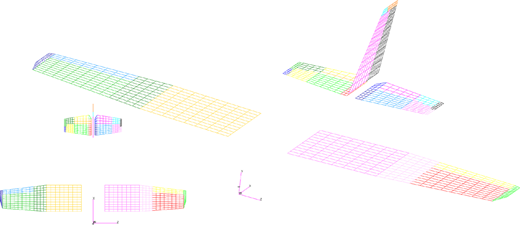
The aeroelastic analysis using MSC.Patran/MSC.Nastran relies on the FE method supplemented with aerodynamic elements, see Figure 10. The primary inputs include the structural stiffness represented by the elastic model, mass and moments of inertia represented by lumped masses, and aerodynamic excitation linked to the elastic model to provide structural excitation.

The p-k method (Hexagon, 2024a), which is widely used to calculate the critical flutter speed, is an iterative process. It is applied for each combination of airspeed, air density and natural mode of the structure. During each iteration, the method solves for complex eigenvalues of the aeroelastic equation of motion equation (7). These eigenvalues provide the damping value g, where zero damping indicates the aeroelastic stability limit of the mode and the corresponding airspeed is the critical flutter speed:

where M_hh is the modal mass matrix, B_hh is the modal damping matrix, K_hh is the modal stiffness matrix, k = ωc\(2v) is the reduced frequency, c is the reference depth, ω is the circular frequency, V is the airspeed, ρ is the air density, $QhhR$ is the modal aerodynamic stiffness matrix and $QhhI$ is the modal aerodynamic damping matrix. These matrices are the real and imaginary components of the aerodynamic force matrix Q_hh and both are functions of the Mach number M and the reduced frequency k. The value of p in equation is the eigenvalue p = ω(γ ± i), where γ is the transient decay rate, which is related to the structural damping coefficient g = 2γ.

Equation (7) is rewritten in state-space form for the p-k method as:

where [A] is real matrix:

and vector {u_h} includes modal displacements and velocities.

The iterative process continues until the difference between the circular frequencies ω obtained in consecutive iterations falls below a specified tolerance, ensuring convergence.

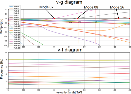
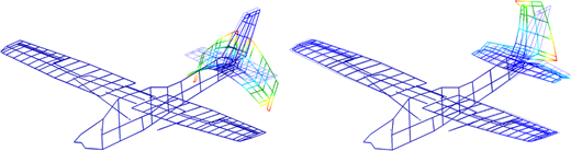
The results of the aeroelastic analysis are presented in the form of v-g and v-f diagrams (velocity-damping and velocity-frequency), which show, for each vibration mode of the aircraft structure, whether the oscillation is damped (g < 0) and flutter does not occur within the given speed range, or undamped. Flutter occurs at the speed where damping reaches zero (g = 0) for a specific vibration mode. The speeds V_NE (never exceed speed), V_D (design diving speed) and V_f (flutter critical airspeed) shown in the graph indicate whether flutter occurs at flight speeds greater than V_f = 1.2 V_D, or below this threshold. Diagram in Figure 11 illustrates that for Modes 7 and 8, flutter occurs at speeds lower than V_f, which is unacceptable from a flight safety perspective, and modifications are required. The shape of these modes is shown in Figure 12. The diagram also shows that for Mode 16, flutter occurs at a speed higher than V_f, providing a sufficient safety margin, so no further action is necessary. For the remaining modes, either flutter does not occur, or it occurs at speeds greater than 450 km/h, which is beyond the studied speed range.

Experience from analyses shows that flutter occurs mostly on unbalanced tail rudders and in the vast majority of cases it is a combination of aft fuselage oscillation and rudder or elevator oscillation. These phenomena can be avoided by at least partially balancing the rudders, thus shifting the flutter speed to higher speeds. This fact is illustrated in Figures 11–13.

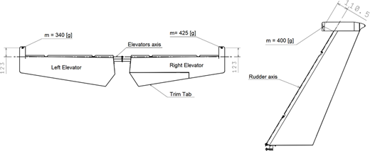
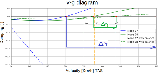
The following v-g diagram (Figure 14) shows the change in flutter speed for the variant without rudder balance and the variant with partial rudder balance (elevator and rudder). Adding mass es in front of the rudder rotation axis, see Figure 13, increased the critical flutter speed from 202 to 339 km/h. Mode 07 even results in complete damping of that mode.

The results of aeroelastic analyses of small sport aircraft highlight the critical importance of accurate input data, particularly stiffness characteristics, for determining the flutter resistance of small aircraft. Ground vibration testing is essential to determine the natural frequencies, mode shapes and damping ratios of the aircraft structure.

Due to the uncertainties in the cross-sectional and material characteristics, especially for composite structures, entering the FE model, it is necessary to perform parametric optimization of these cross-sectional characteristics to achieve agreement between the GVT results and the modal analyses of the aircraft model entering the flatter analysis. Under these conditions, the critical flutter speed can then be correctly determined.

Other findings from the flutter analyses performed (see chapter Effect of control balance) show that flutter occurs predominantly in unbalanced control surfaces such as rudders, and can be mitigated or eliminated completely by balancing, or at least partially balancing (adding mass across the axis of rotation of the rudder) these surfaces, effectively shifting the flutter rate to higher, safer values. These findings highlight the need for accurate control surface balancing and thorough testing to ensure aeroelastic safety in small aircraft designs.

A potential extension of this method is its application to other aircraft categories, including general aviation aircraft and unmanned aerial vehicles.

This work was supported by the project No. FSI-S-23-8163 funded by The Ministry of Education, Youth and Sport (MEYS, MŠMT in Czech) institutional support.