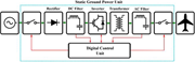
Figure 1 Schematic diagram of a conventional static aircraft ground power unit Source: Authors’ own work A block diagram shows a static ground power unit converting and controlling electrical power before supplying an aircraft. The block diagram represents a Static Ground Power Unit connect... More about this image found in Schematic diagram of a conventional static aircraft ground power unit Sou...

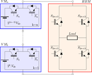
Figure 2 Cascaded asymmetric multilevel inverter topology Source: Authors’ own work A circuit diagram connects cascaded V M modules to an H B M containing four switches and a central load. The circuit diagram contains a cascaded V M structure on the left and an H B M on the right. The upper... More about this image found in Cascaded asymmetric multilevel inverter topology Source: Authors’ own wo...

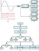
Figure 3 Switching control framework: (a) switching strategy of 15-level waveform and (b) signal generation block diagram and (c) signal generation flowchart Source: Authors’ own work Three panels present a stepped output waveform, switching signals S 1 to S 5, switching logic, and the corre... More about this image found in Switching control framework: (a) switching strategy of 15-level waveform an...

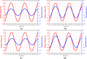
Figure 4 Simulated output waveforms of the proposed 31-level inverter under different load conditions: (a) R = 27.43 Ω, (b) R = 16 Ω, (c) Z_L = 30.11 + j7.54 Ω, (d) Z_L = 15.63 + j5.33 Ω Source: Authors’ own work Four dual-axis line graphs plot output voltage and load current against time from 17 to 23 milliseconds. In every panel, the horizontal axis is Time in milliseconds from 17.0 to 23.0, with labelled intervals of 0.5 milliseconds. The left vertical axis is Output Voltage in volts, ranging from negative 200 to 200 at intervals of 50 volts. The right vertical axis is Load Current in amperes, ranging from negative 20 to 20 at intervals of 5 amperes. Panel a has a stepped output-voltage waveform that rises from about negative 150 volts at 17.0 milliseconds, crosses 0 near 17.5 milliseconds, reaches about 160 volts near 18.1 milliseconds, crosses 0 near 18.8 milliseconds, reaches about negative 160 volts near 19.4 milliseconds, crosses 0 near 20.0 milliseconds, reaches about 160 volts near 20.6 milliseconds, crosses 0 near 21.3 milliseconds, reaches about negative 160 volts near 21.9 milliseconds, and rises towards about 150 volts at 23.0 milliseconds. The load current follows the same oscillatory timing, with peaks near 6 amperes and troughs near negative 6 amperes. Panel b has a stepped output-voltage waveform with positive peaks near 155 volts around 18.1 and 20.6 milliseconds and negative troughs near negative 155 volts around 19.4 and 21.9 milliseconds. Its load current follows the oscillation with positive peaks near 10 amperes and negative troughs near negative 10 amperes. Panel c has a stepped output-voltage waveform with positive peaks near 160 volts around 18.1 and 20.6 milliseconds and negative troughs near negative 160 volts around 19.4 and 21.9 milliseconds. Its load current has positive peaks near 6 amperes and negative troughs near negative 6 amperes, following the output-voltage oscillation. Panel d has a stepped output-voltage waveform with positive peaks near 155 volts around 18.1 and 20.6 milliseconds and negative troughs near negative 155 volts around 19.4 and 21.9 milliseconds. Its load current reaches approximately 10 amperes at its positive peaks and negative 10 amperes at its negative troughs. In panel d, the load-current waveform is visibly displaced in time relative to the output-voltage waveform, with its peaks and troughs occurring slightly after the corresponding voltage peaks and troughs. Each panel covers approximately two complete oscillations between 17.0 and 23.0 milliseconds. More about this image found in Simulated output waveforms of the proposed 31-level inverter under differen...

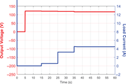
Figure 5 Transient response of the proposed 31-level inverter under sequential load variations Source: Authors’ own work A dual-axis line graph plots stepped output voltage and load current over 60 seconds, with both increasing at specified times. The dual-axis line graph plots output volta... More about this image found in Transient response of the proposed 31-level inverter under sequential load ...

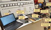
Figure 6 Experimental setup for performance evaluation of the proposed 31-level inverter Source: Authors’ own work A laboratory test setup labels a host P C, power supply, 31 level inverter, battery modules, analysers, probes, and R L load banks. The laboratory test setup contains multiple ... More about this image found in Experimental setup for performance evaluation of the proposed 31-level inve...

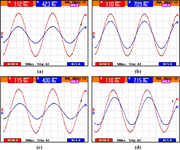
Figure 7 Experimental output waveforms of the proposed 31-level inverter under different load conditions:(a) R = 27.43 Ω, (b) R = 16 Ω, (c) Z₁ = 30.11 + j7.54 Ω; (d) Z₁ = 15.63 + j5.33 Ω Source: Authors’ own work Four oscilloscope panels compare voltage and current waveforms, with R M S voltage near 110 volts and current from 4.00 to 7.15 amperes. Each panel contains channel A and channel B periodic traces across a dotted grid. Each display has B W L 10 kilohertz and HOLD at the top, and A equals 50 volts, 500 microseconds, Trig: A J, and B equals 5 amperes along the bottom. Channel A and B reference markers appear beside the traces and at the right edge. Panel a displays channel A at 112 volts R M S and channel B at 4.23 amperes R M S. Channel A has a larger vertical trace amplitude, while channel B has a smaller amplitude and its peaks and troughs occur slightly after those of channel A. Approximately two complete cycles and part of a third are visible. Panel b displays channel A at 110 volts R M S and channel B at 7.09 amperes R M S. Channel A and B have similar periods, with their peaks, troughs, and zero crossings occurring close together. Approximately two complete cycles and part of a third are visible. Panel c displays channel A at 115 volts R M S and channel B at 4.00 amperes R M S. Channel A has a larger vertical trace amplitude, while channel B has a smaller amplitude and its peaks and troughs occur slightly after those of channel A. Approximately two complete cycles and part of a third are visible. Panel d displays channel A at 110 volts R M S and channel B at 7.15 amperes R M S. Channel A and B have similar periods, with channel B peaks and troughs occurring slightly after those of channel A. Approximately two complete cycles and part of a third are visible. A small J marker appears near the right side of panel d. More about this image found in Experimental output waveforms of the proposed 31-level inverter under diffe...

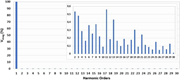
Figure 8 Harmonic spectrum of the proposed 31-level inverter under resistive load condition (R = 27.43 Ω) Source: Authors’ own work A bar chart shows the percentage magnitude of harmonic orders 1 to 30, with the first harmonic dominant and higher harmonics below 0.6 per cent. The bar chart ... More about this image found in Harmonic spectrum of the proposed 31-level inverter under resistive load co...

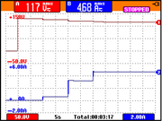
Figure 9 RMS voltage and current variations of the proposed 31-level inverter under sequential load variations Source: Authors’ own work An oscilloscope display presents stepped voltage and current traces, with R M S readings of 117 volts and 4.68 amperes. The oscilloscope display contain... More about this image found in RMS voltage and current variations of the proposed 31-level inverter under...

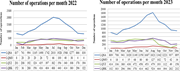
Figure 1 Trend of aircraft operation Source: Bosnia and Herzegovina Air Navigation Services Agency (BHANSA), 2025 Two-line graphs compare monthly operations for L Q S A, L Q M O, L Q T Z, and L Q B K in 2022 and 2023. The two-line graphs have the titles Number of operations per month 2022 ... More about this image found in Trend of aircraft operation Source: Bosnia and Herzegovina Air Navigatio...

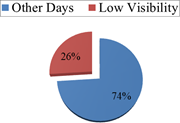
Figure 2 Percentage of days with low visibility in December 2022 Source: Bosnia and Herzegovina Directorate of Civil Aviation (BHDCA), 2023 A pie chart depicts the Percentage of days with low visibility in December 2022. The pie chart contains two categories. Low Visibility accounts for 26... More about this image found in Percentage of days with low visibility in December 2022 Source: Bosnia a...

Figure 3 Analysis of the missed approach according to the current 2.5% climb gradient procedure Source: Author’s own work A Three-dimensional terrain view compares current O C A slash H with C A T 3 minimum and a 2.5 per cent climb gradient. The three-dimensional terrain view shows an airpo... More about this image found in Analysis of the missed approach according to the current 2.5% climb gradien...

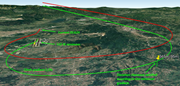
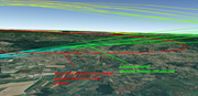
Figure 4 The current missed approach procedure (marked in red) and radar paths of aircraft, November 2023 (marked in green) Source: Author’s own work A Three-dimensional terrain view compares a missed-approach procedure with radar tracks showing climb gradients between 10 and 18 per cent. T... More about this image found in The current missed approach procedure (marked in red) and radar paths of ai...

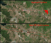
Figure 5 Approach and take-off surfaces at LQTZ Source: Author’s own work Two satellite views show airport approach and take-off climb surfaces outlined across the surrounding terrain. Two stacked satellite views show an airport and surrounding terrain. The upper view is titled Approach S... More about this image found in Approach and take-off surfaces at LQTZ Source: Author’s own work Tw...

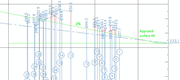
Figure 6 Obstacles in the approach surface for Runway 09 Source: AIP BiH, 2025 A Profile chart shows a 2 per cent Approach surface 09 with numbered obstacles and elevation values along the descending surface. The profile chart shows Approach surface 09 as a descending line marked 2 per cen... More about this image found in Obstacles in the approach surface for Runway 09 Source: AIP BiH, 2025 ...

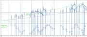
Figure 7 Obstacles in the approach surface for Runway 27 Source: AIP BiH, 2025 A Profile chart shows 2 per cent Approach surface 27 with 53 numbered obstacles and multiple elevation profiles. The profile chart shows Approach surface 27 with a rising 2 per cent surface line, a lower rising ... More about this image found in Obstacles in the approach surface for Runway 27 Source: AIP BiH, 2025 ...

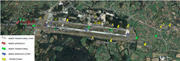
Figure 8 Penetration points into the OFZ Source: Author’s own work A Satellite view of Tuzla International Airport shows runway 09 and marked obstacles including trees, masts, buildings and approach areas. The satellite view shows Tuzla International Airport, the runway and surrounding fi... More about this image found in Penetration points into the OFZ Source: Author’s own work A Satelli...