Air pollution from gas flaring: a diachronic assessment in an Algerian oil field

The process of Oil & Gas extraction and processing generates an important volume of natural gas. The latter is burned due to the high economic costs of recovery and safety considerations. This disposal process is called Gas Flaring (GF) (Faruolo, Caseiro, Lacava, & Kaiser, 2021; Hu, Zhang, Xing, & Gao, 2023; Khreebsh & Azeez, 2024). GF exists at all levels of Oil & Gas industry and is used to vent several types of continuous, Operational and start-up waste gases (Anejionu, 2019). In this regard, continuous flaring is used in oil extraction industry where the cost of gas valorization is economically high. The operational GF is conducted when a technical problem happens in an oil & gas installation and the latter must be depressurized for safety reasons (Faruolo et al., 2021). As for the start-up GF, it is conducted during start-ups or shutdowns of an installation during a planned maintenance (Ahmadi, Minaei, Ebadollahi, Ghaebi, & Shahrivar, 2023; Anejionu, 2019).

The World Bank estimates that 144 billion m³ was burned in 2021, emitting approximately 0.4 billion tons of carbon dioxide (CO₂) (GGFR, 2022). The latter is considered the most present greenhouse gas in the atmosphere (Kamali Saraji, Streimikiene, & Balezentis, 2025; Lan et al., 2020). However, the impact of flaring in terms of global warming cannot be only reduced to this number. In fact, the efficiency of GF is generally between 97 % and 98 %. This means that 2% to 3% methane is released unburned. It should be noted that a methane molecule released in place of a CO₂ molecule have a 28 times higher global warming potential. Consequently, the impact of GF is increased by 50% to 75% regarding global warming (Faruolo et al., 2021; Ialongo, Stepanova, Hakkarainen, Virta, & Gritsenko, 2021). Furthermore, GF emits a number of polluting gases (e.g. SO₂, NO_X, PM, CO_X) that alter the air quality of surrounding areas and consequently cause respiratory diseases for workers and residents who are exposed for a considerable amount of time (Aczel & Makuch, 2020; Franklin, Chau, Cushing, & Johnston, 2019; Shojaei, Vahabpour, Saifoddin, & Ghasempour, 2023; Bouras et al., 2024).

In 2015, the “Zero Routine Flaring initiative” (ZRF) was launched by the World Bank and the UN Secretary General setting goals for 2030. In this regard, more than 80 countries and oil companies have ratified the convention and agreed to its commitments including the reduction of GF (GGFR, 2022).

The main emitters of flared gas, by volume, have for nine consecutive years been in approximately the following order, the Russian Federation, Iraq, the Islamic Republic of Iran, the United States, Algeria, the Republic Bolivia, Republic of Venezuela and Nigeria. These countries are, jointly, responsible for 40% of the world's annual oil production, but around 65% of the volume of gas flared (GGFR, 2022; Harrison & Sahel, 2023).

It should be noted that Algeria possesses the 10th largest natural gas reserves and is considered as the 4th largest gas exporter in the world. It also ranks 16th in terms of crude oil reserves and it exports over 60% of its production (Álvarez, 2010). This has led Algeria to hold the 5th place in GF with an estimated quantity of 8614,02 Million m³/Year (GGFR, 2022). In this regard, Algeria has endorsed in 2018 the initiative of World Bank's ZRF by 2030 (GGFR, 2022). National regulations were also proposed by the Algerian government such as the Law No. 19–13 that covers all matters pertaining to oil and gas activities, including abandonment, flaring, and environmental issues. The latter law is enforced by 2 agencies that are the Hydrocarbon Regulation Authority (ARH) and the National Agency for Valuation of Hydrocarbon Resources (ALNAFT) (Álvarez, 2010).

Therefore, Algerian companies are obligated to reduce their environmental GF impact to respect applied laws. For this, detailed information must be provided about the volumes of flared gas as well as the quantity of pollutant emissions and their dispersion. In this regard, a number of models that assess the dispersion of pollutant gases emitted by flaring have been proposed. These models combine meteorological conditions and atmospheric layer heights to give an approximate dispersion model. It should be noted that Computational Fluids Dynamics (CFD), Gaussian plume, Lagrangian particle and chemical transport are the most used models in the scientific literature with a certain preference for the Lagrangian one (Zhang & Wang, 2022).

Furthermore, the evaluation of flared gases volumes also relies on remote sensing techniques such as VIIRS (The Visible Infrared Imaging Radiometer Suite) refined by linear and non-linear spectral unmixing techniques (Benhalouche, Benharrats, Bouhlala, & Karoui, 2022).

These tools and models must be framed by a GF assessment study such as the diachronic approach chosen in this article. As a reminder, any diachronic study is framed by the concept of “synchrony-diachrony” used in many fields more particularly in environmental studies (Dietrich, 2020; Winter, 2024).

Furthermore, a diachronic study is a comparison of two or more synchronic studies. Thus, the concept of “synchrony-diachrony” makes it possible to consider and articulate the two approaches to obtain a more complete and nuanced understanding of the phenomena studied (Winter, 2024). Its interest is to highlight changes (trends) in a well-defined phenomenon (i.e. dynamics of environmental degradation, dynamics of environmental restoration, etc.) (Siba, Aboura, Kechairi, Maatouk, & Sebbah, 2024).

In the context of atmospheric pollution in Algeria, existing studies have primarily focused on synchronic assessments, often based on short-term measurements or single-year analyses. For example, Bouras et al. (2024) assessed atmospheric pollution around the Skikda LNG complex using in situ measurements of major pollutants (e.g. CH₄, CO₂, SO₂, and NO_x). They found elevated methane and carbon monoxide concentrations near the site that exceeded the Algerian permissible limit. However, no previous study has applied a diachronic modeling approach to assess gas flaring emissions and their atmospheric dispersion using dedicated simulation tools in Algeria.

To fill this gap, this study introduces a diachronic (2018–2022) and seasonal (i.e. four climatological scenarios per year) modeling design for gas flaring dispersion in Algeria using the Hybrid Single-Particle Lagrangian Integrated Trajectory (HYSPLIT). This is conducted by integrating validated operator flaring-volume data with transport/dispersion modeling to connect operational variability to the atmospheric footprint. Also, it provides quantitative envelopes of horizontal and vertical plume reach after 72 hours, clarifying when and how flaring emissions may become transboundary.

Consequently, its aim is to sustain the actions of GF reduction in a large Algerian oil & gas field by linking its findings to concrete policy objectives, such as Algeria's endorsement of the World Bank's ZRF by 2030 initiative.

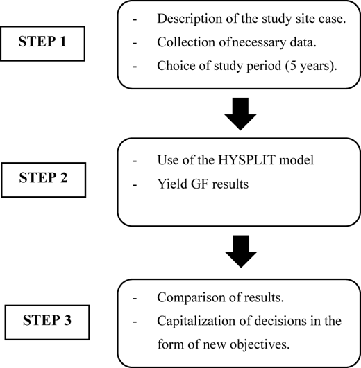
The general methodology of the present diachronic study is based on three main steps detailed below (Figure 1).

1. Step 1 = The starting point is the description of the “Study Area”. The choice of this area is conditioned by two main criteria, namely the representativeness of the phenomenon studied and the availability of the data to be used. The availability of data to be retained in a diachronic study inevitably leads to the choice of the study period which materializes the diachronic approach. Indeed, a diachronic approach focusing on the dynamics of a phenomenon (such as an environmental issue) presents at least two study periods, one “upstream” and the other (or others) “downstream”, making it possible to affirm (or refute) the trend of the obtained results.

   Therefore, the choice of periods in a diachronic study is of great importance: on the one hand, they allow us to justify the upstream period taking into account the availability of data and their representativeness of the environmental problem (e.g. peak period of flared gas discharges) and, on the other hand, they allow us to justify the dynamics of this problem over a time range considered representative. As a reminder, this time range often consists of a couple of years (e.g. 5 Years) (Tümtürk, Karakiewicz, & de Haan, 2024).

2. Step 2 = The second step of a diachronic study concerns the choice of the comparison method between the study periods of a phenomenon. In this regard, the most widely used methods in diachronic studies of environmental issues are Cost-Benefit Analysis (CBA) (Kozlovsky & Feniger, 2021; Vanderlinden, Rouhaud, & Touili, 2022), satellite imagery by GIS (Siba et al., 2024) or simulations using appropriate computer tools (Zhang & Wang, 2022). It is important to remember that each of these methods has multiple variants. Thus, for the CBA, it relates to the analysis of avoided damage and cost-effectiveness analysis.

   As for GIS, it concerns essentially cartographic and digital terrain models that are the most deployed. As for simulation tools, these are dynamic models such as the HYSPLIT tool which continues to be one of the most widely used atmospheric transport and dispersion models in the atmospheric science community (Jooybari, Peyrowan, Rezaee, & Gholami, 2022; Ma et al., 2021). It is for this reason that this tool is retained in the remainder of this study.

3. Step 3 = The third and final step concerns the interpretation of the results obtained by taking into account the objective of the study and proposal of corrective measures.

Hassi R'mel oil field is located north of the Algerian Sharan platform. It is located between the meridians 2°55′ and 3°45′ East and the parallels 33°15′ and 33°45 North at an altitude of 760 m. Hassi R'mel covers an area of more than 3500 km² and is considered an important deposit of natural gas, condensate and LPG, estimated at 200 g/m³ for condensate, 80 g/m³ for LPG and a minimal fraction of oil (crude oil) in the “Eastern” and “South” parts of the field. The region of Hassi R'mel is composed of 3 parts (i.e. North, South and Center). The center part is considered as the largest as it contains: 1 Boosting Center Station (BCS), 3 Gas Module Processing Plant (MPP0, MPP1, MPP4), 1 Common Unit for Modules MPP0 and MPP1 (phase B), 1 Storage and transfer center (CSTF), 1 Associated gas recovery station (SRGA) and 2 Oil Treatment Center (CTH1, CTH2).

To estimate the trajectory and dispersion of pollutants generated by GF, a diachronic study was conducted using HYSPLIT for MPP4. The latter was selected considering the availability of operational data. In this regard, seasonal simulations were performed for each year of the study period (2018–2022). It should be noted that the selected period corresponds to the years for which validated GF data were available from the site operator. Data from 2023 onward were not yet accessible at the time of the study.

For each year of the studied period, four representative simulations were conducted by selecting the mid-season date of each climatological season (i.e. winter: 15 January; spring: 15 April; summer: 15 July; autumn: 15 October). Each simulation consisted of a 72-hour forward run at 100 m above ground level (AGL), initialized at 00:00 UTC. This standardized seasonal sampling repeated across multiple years is intended to isolate systematic seasonal transport behavior while still capturing interannual variability, which is the central added value of the diachronic approach adopted here.

Meteorological input data were obtained from the NOAA Global Data Assimilation System (GDAS) with a horizontal resolution of 1°, providing three-dimensional fields of wind, temperature, and boundary-layer parameters required for trajectory and dispersion calculations.

The HYSPLIT tool is a complete system allowing the calculation of simple trajectories of air masses, as well as complex simulations of transport, dispersion, chemical transformation and deposition of gaseous pollutants or particles (Kozlovsky & Feniger, 2021). It was developed by National Oceanic and Atmospheric Administration (NOAA) and the Air Resources Laboratory (ARL) in the USA (Hu et al., 2023; Stein et al., 2015).

It should be noted that HYSPLIT is based on a hybrid calculation approach using Eulerian and Lagrangian approaches. The former calculates the concentrations using a fixed grid meaning that the model uses the integration of pollutant flows at each grid cell interface due to advection and diffusion. Subsequently, advection and diffusion are carried out in a Lagrangian framework (Hu et al., 2023; Schade & Gregg, 2022).

The Lagrangian model is considered efficient and flexible. This is due to the fact that it can calculate the dispersion of discrete puffs and pollutant's particles through complex wind fields. This allows the simulation of pollutants transport over topographical changes. In addition, the Lagrangian model can be applied to situations with varying parameters (i.e. temporal, spatial, meteorological). This has led for the Lagrangian model to be widely used in the scientific literature (Draxler & Hess, 1998; Schade & Gregg, 2022).

Furthermore, HYSPLIT tool is based on the calculation of Advection and Diffusion. The former is calculated from the mean position of the three-dimensional velocity vector between the initial position $P(t)$ and the first approximation position $P′(t+Δt)$ (Draxler & Hess, 1998; Escudero et al., 2006). The mean velocity vectors $V$ are linearly interpolated in space and time. This leads us to the first approximative position:

To estimate concentrations, it is essential to trace individual particles or determine their distribution along the mean trajectory. This is achieved by introducing a random component to the average advection velocity, which characterizes the dispersion of the pollutant plume. For instance, horizontal particle dispersion can be described using the following equations:

Where: $U′$ is the Random Velocity Component, $Xmean$ is the Initial position due to only advection by wind speed, $R$ is the Autocorrelation of turbulent speed, $σi$ is the Standard deviation of turbulent speed, $Tlx$ is the Lagrnagian constant and $λ$ is the Computer-generated number between 0 and a mean σ of value equal to 1.

The calculations can be simplified by calculating the mean particle trajectory position and particle distribution instead of modeling the motion of each particle. The standard deviation of particle's distribution can be calculated from all particles:

With: $Xi$ is the Position of particle $i$ and $Xm$ is the mean position

Eq. (8) represents the particle distribution (i.e. Puff Mode) in which the horizontal standard deviation of the particles is given as:

The dispersive growth rate of particles or puffs is controlled by the standard deviation of the turbulent velocity. Eq. (9) represents the simplified used in HYSPLIT:

Air concentrations are determined by summing the mass of individual particles as they pass through the concentration grid. In the 3-D particle model mode, this grid is conceptualized as a matrix of cells, each defined by specific spatial dimensions. Consequently, the concentration increment at a given cell is calculated as the particle mass divided by the volume of that cell:

In hybrid mode, the vertical component of the concentration is still computed based on the depth of each grid cell. However, the horizontal dimension is represented by a network of nodes rather than continuous cells. If a node lies within the particle distribution, the concentration at that node is then calculated accordingly.

Two distinct approaches can be used to represent horizontal distributions. In the conventional Gaussian (GS) formulation, the concentration change contributed by a puff at each grid point is calculated as follows:

An alternative representation is the simplified Top Hat (TH) model, where each grid point is considered either entirely within the puff or entirely outside of it. Within the puff, the concentration is assumed to be uniform and equal to the average concentration of the corresponding Gaussian distribution:

Furthermore, equations used for this study with further explanations can be found in NOAA's publications on HYSPLIT (Draxler & Hess, 1997, 1998; Stein et al., 2015).

It should be noted that HYSPLIT is used to infer pollutant transport dynamics and relative concentration distributions under realistic atmospheric conditions. As such, the results should be interpreted as representative estimates of dispersion trends and spatial influence rather than absolute concentration values.

This approach is used in atmospheric pollution studies and is particularly suitable for regions where continuous ground-based monitoring is limited (Enciso-Díaz, Zafra-Mejía, & Hernández-Peña, 2025).

Results from the diachronic study orient decision-makers to implement actions in relation to GF. More precisely, it is a question of comparing GF according to the studied periods. This comparison makes it possible to decide on the objective that frames GF. Thus, if this objective is achieved at the end of the diachronic study, the decision must be focused on its sustainability for the post-diachronic study. On the other hand, if this objective is not achieved, the decision to be made makes it possible to redefine a new objective of GF for the future.

For a better definition of this future time horizon relative to the new objective, it is imperative to take into consideration the hazards that may accompany the achievement of this new objective. Hence the interest in considering two future horizons (or durations): an optimistic duration (d_o) and another pessimistic one (d_p) which takes into account possible hazards (Saadi, Djebabra, & Boubaker, 2011).

In this regard and in the case where the probability of achieving the new objective in the near future ([d_p – d_o]) follows a normal distribution, Boulagouas, Chaib, and Djebabra (2021) state that the most probable future horizon (d_x) is expressed by:

In Eq. (13) d_m is the mean duration (i.e. mean horizon between d_o and d_p). Thus, and taking into account the nature of the probabilistic law of duration (d_x), its variance (V) is expressed by:

GF is identified as the main source of atmospheric pollution in the Hassi R'mel central region. Flared gas is predominantly composed of methane, along with other light hydrocarbons and impurities, while GF emissions inlcude atmospheric pollutants (e.g. CH4, CO, SO2, and NOx). The annual volumes of flared gas expressed in standard cubic meters (sm³) were calculated based on operational data provided by the operator of MPP4 (Table 1). Furthermore, flared gas volumes were determined from continuous monitoring records of the flare system, which register gas flow rates directed to flaring during routine operations, maintenance events, and unplanned upsets.

The data in Table 1 show that there is no proportionality between the quantity of produced and flared gas during the same year. These same data also show that the flared gas threshold is reached in 2019. To assess the atmospheric implications of these interannual variations, dispersion simulations were conducted using HYSPLIT model.

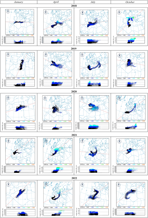
Simulations were performed for representative dates corresponding to the four climatological seasons (i.e. winter, spring, summer, and autumn) for each year between 2018 and 2022. This yielded a total of 20 simulations (Figure 2). Each simulation consisted of a 72-hour forward run with emissions released at 100 m AGL from the oil field considered as the source zone (The source zone is represented by a red star).

Estimated distances of horizontal and vertical extents of gas flaring plumes after 72 hours for each season and year of were inferred from HYSPLIT particle dispersion maps (Table 2).

In addition, simulated mean concentrations of the major flaring-related pollutants (CO₂, CH₄, SO₂, and NO_x) were obtained (Table 3). Concentrations are expressed in µg/m³ for SO₂ and NO_x, and in ppm for CH₄ and CO₂. The values represent the range of near-field (<10 km) and far-field (>100 km) concentrations averaged over the study period.

The present study provides a diachronic and seasonal evaluation of gas flaring (GF) dispersion dynamics in the Hassi R'mel region based on HYSPLIT simulations spanning 2018–2022.

An examination of Table 1 reveals a clear temporal segmentation of the 2018–2022 period into two distinct phases characterized by contrasting gas flaring (GF) behaviors.

The first phase (2018–2019) is marked by a sharp increase in flared gas volumes, rising from 8,681 × 10³ sm³ in 2018 to 26,380 × 10³ sm³ in 2019, corresponding to an increase factor of approximately 3.0 (+204%). This increase is not correlated with a comparable rise in gas production, indicating that flaring intensity during this period was driven primarily by operational constraints (i.e. Maintenance activities) rather than production demand (Anejionu, 2019; Nwagbara, 2020).

The second phase (2020–2022) exhibits a sustained decline in GF volumes, followed by stabilization at significantly lower levels. Flared gas quantities decreased to 5,024 × 10³ sm³ in 2020, before stabilizing at 9,069 × 10³ sm³ in 2021 and 6,808 × 10³ sm³ in 2022. When compared to 2019, this represents a reduction of approximately 81% in 2020, 66% in 2021, and 74% in 2022. This reduction is consistent with the company's efforts to meet the World Bank's ZRF that Algeria ratified (GGFR, 2022). The achievement of this objective over the 2018–2022 horizon suggests a positive shift toward operational efficiency and environmental protection.

HYSPLIT simulations consistently indicate a prevailing east to northeast transport direction, with plume extents ranging from regional (300–600 km) to transboundary scales (>800 km) within 72 hours (Table 2). In this regard, short horizontal reaches are associated with winter conditions that are characterized by weaker wind speeds and more stable atmospheric conditions. As for spring and summer simulations, they exhibit the largest plume extensions due to stronger synoptic winds and enhanced atmospheric mixing (Mamtimin et al., 2020).

Interannual differences in horizontal reach are comparatively minor. This suggests that meteorological conditions exert a stronger control on plume transport than year-to-year variations in GF volumes (Jury & Gaviria Pabón, 2021). Furthermore, the trajectory results confirm that GF emissions from the Hassi R'mel region have the potential to affect distant areas well beyond the source, reinforcing the regional and cross-border nature of their environmental impact (Halkos & Tsilika, 2019). This finding can only be obtained from a diachronic comparison where it shows that seasonality is the primary driver of long-range footprint, whereas interannual changes in flaring volume mainly modulate near-field intensity.

The HYSPLIT dispersion simulations provide insight into the spatial extent and vertical development of GF plumes (Figure 2 & Table 2). Across the 2018–2022 period, dispersion patterns consistently show higher pollutant retention in the near-field zone during early stages, followed by progressive spatial expansion. This reflects the combined influence of atmospheric turbulence and wind patterns governing plume evolution.

The dispersion results are consistent with the horizontal reach summarized in Table 2, which indicate that plume spreading increases substantially after 72 hours, particularly during spring and summer seasons. Conversely, winter simulations are characterized by more compact dispersion patterns, reflecting stable atmospheric conditions that favor localized pollutant buildup (Jury & Gaviria Pabón, 2021).

It should be noted that absolute pollutant concentrations decrease with distance from the source. Nevertheless, modeled dispersions demonstrate that GF emissions can influence air quality over regional scales. Consequently, a reduction in GF translates into a reduced spatial footprint. This reinforces the importance of sustained flaring mitigation strategies for limiting both local and regional environmental impacts (Haleem Ali Al Muhyi & Younis Khalil Aleedani, 2023).

The simulated concentrations of CO₂, CH₄, SO₂, and NO_x (Table 3) show distinct differences between near-field (<10 km) and far-field (>100 km) environments, reflecting the combined influence of combustion intensity and dispersion dynamics.

In this regard, SO₂ and NO_x concentrations reached indicative mean range of 85–140 µg/m³ near the flaring zone. These estimated concentrations are comparable to those reported near oil and gas facilities in similar arid environments (Fawole, Cai, & MacKenzie, 2016; Haleem Ali Al Muhyi & Younis Khalil Aleedani, 2023). Nevertheless, these values may exceed guideline values (24 Hours Means) defined by international air quality guidelines (i.e. 40 µg/m³ for SO₂ and 25 µg/m³ for NO₂) (WHO, 2021).

Furthermore, estimated far-field values decline significantly to 25–50 µg/m³ for SO₂ and NO_x, demonstrating efficient atmospheric dilution under the region's typical wind regimes. Nevertheless, chronic exposure to even low concentrations of flared pollutants (e.g. SO_x, NO_x, etc.) has been linked to adverse health outcomes, such as respiratory and cardiovascular diseases (Pérez Velasco & Jarosińska, 2022).

The modeled concentrations of greenhouse gases “CO₂” and “CH₄” show smaller spatial gradients, with near-field averages of 420–480 ppm and 2.4–3.0 ppm. Although these values remain within global background ranges, their persistence highlights the site's contribution to Algeria's total greenhouse gas inventory (GGFR, 2022).

Based on the analysis of the spatial dispersion patterns and modeled concentrations of GF pollutants, the reduction achieved by 2022 provides a reference point for defining more mitigation objectives over the subsequent period (2023–2030). Any future target should be framed within the dual context of minimizing the loss of a non-renewable energy resource and limiting local and regional environmental impacts.

Using the probabilistic framework described in Eq. (13) and Eq. (14) with a lower bound “d_o = 2026” and an upper bound “d_p = 2030”, the estimated timeframe for achieving the revised objective corresponds to “d_x = 2028” with a low variance “V = 0.44” indicating moderate uncertainty. This suggests that the Hassi R'mel field is statistically most likely to reach its flaring minimization goal around 2028, assuming current mitigation efforts continue at their present pace. Indeed, potential flare malfunctions and unplanned operational events remain plausible in oil and gas operations and must be explicitly accounted for when defining long-term mitigation trajectories (Lopez, Saud, & Vaez, 2015).

The study's findings are transferable to other Oil & Gas production regions that share similar environmental, meteorological, and industrial characteristics as the Hassi R'mel region. In particular, fields in arid or semi-arid climates with prevailing seasonal wind patterns (e.g. North Africa, Middle East, and parts of Central Asia). Theoretically, the diachronic–seasonal framework demonstrates the added value of separating the influence of seasonal meteorology from interannual operational variability. This provides a more robust interpretation of flaring dispersion than single-period snapshots.

Practically, the applied approach offers a replicable framework for long-term environmental monitoring. In this regard, the recurrent east–northeast transport pathway provides a defensible basis for targeted monitoring placement and for designing near-field versus far-field observation strategies. Overall, the approach offers a decision-support template for local governments, regulators, and stakeholders in identifying critical time periods and implementing mitigation strategies. It can be applied by any country pursuing emission reduction goals aligned with the World Bank's ZRF initiative.

This study provides a comprehensive assessment of gas flaring (GF) emissions in the Hassi R'mel region in Algeria and their atmospheric dispersion over the 2018–2022 period. By combining interannual flaring data with seasonal HYSPLIT simulations, the analysis highlights the potential environmental and human exposure implications associated with GF-related pollutants (e.g. CO₂, CH₄, SO_x, and NO_x). The modeling results demonstrate that, while GF emissions initially exert a strong local influence, their dispersion over a 72-hour period frequently extends toward the east and northeast, affecting eastern Algeria, neighboring countries and, in some cases, the Mediterranean basin.

These findings confirm the regional and transboundary nature of GF impacts and underscore the importance of addressing flaring as more than a strictly local environmental issue. Therefore, policymakers, industry and stakeholders are required to formulate targeted interventions and regulations aimed at minimizing the adverse effects at a national and regional scales. Future research should aim to strengthen the robustness of modeled estimates through the integration of field measurements, satellite observations, or regional air quality monitoring networks.

It should be noted that the diachronic study, like any modeling-based assessment, has limitations that must be taken into account when evaluating the results:

1. The first is based on the interpretation of digitized dispersion outputs generated by the HYSPLIT model. These outputs represent simulated atmospheric transport patterns that are sensitive to meteorological environmental factors. Consequently, the results should be interpreted in terms of the spatial and temporal evolution of dispersion envelopes, rather than as exact representations of real-time concentration.

2. A second limitation concerns the study period which, in the case where it is very short or too long, can affect the reliability of the data retained. Thus, it is accepted that for certain periods of diachronic studies the dynamics of the observed phenomenon is more “one-off” than truly “trend-based”. In this regard, (Jooybari et al., 2022) suggests focusing on global trends or using “indicator values” with reference to a simple but operational periodicity.

AGL

Above Ground Level

CBA

Cost-Benefit Analysis

GF

Gas Flaring

HYSPLIT

Hybrid Single-Particle Lagrangian Integrated Trajectory

MPP4

Module Processing Plant 4

NOAA

National Oceanic and Atmospheric Administration

ZRF

Zero Routine Flaring

The authors thank the reviewers for their insightful comments and constructive suggestions, which substantially improved the clarity and quality of this manuscript.