


This study aims to determine shoreline change statistics and net erosion and accretion, along the Kuakata Coast, a magnificent sea beach on Bangladesh’s southernmost point.
The research follows a three stages way to achieve the target. First, this study has used the geographic information system (GIS) and remote sensing (RS) to detect the temporal observation of shoreline change from the year 1991 to 2021 through satellite data. Then, the digital shoreline analysis system (DSAS) has also been explored. What is more, a prediction has been done for 2041 on shoreline shifting scenario. The shoreline displacement measurement was primarily separated into three analytical zones. Several statistical parameters, including Net Shoreline Movement (NSM), Shoreline Change Envelope (SCE), End Point Rate (EPR) and Linear Regression Rate (LRR) were calculated in the DSAS to quantify the rates of coastline movement with regard to erosion and deposition.
EPR and LRR techniques revealed that the coastline is undergoing a shift of landward (erosion) by a median rate of 3.15 m/yr and 3.17 m/yr, respectively, from 1991 to 2021, 2.85 km2 of land was lost. Naval and climatic influences are the key reasons for this variation. This study identifies the locations of a significantly eroded zone in Kuakata from 1991 to 2021. It highlights the places that require special consideration while creating a zoning plan or other structural design.
This research demonstrates the spatio-temporal pattern of the shoreline location of the Kuakata beach, which would be advantageous for the region’s shore management and planning due to the impacts on the fishing industry, recreation and resource extraction. Moreover, the present research will be supportive of shoreline vulnerability. Hence, this study will suggest to the local coastal managers and decision-makers for particularizing the coastal management plans in Kuakata coast zone.
1. Introduction
A shoreline is a physical barrier between land and the sea or another body of water. A coast in physical oceanography is the larger fringe that has been geologically transformed mostly by the impact of the water body and a distinct geologic, ecological and biological zone that supports a wide variety of aquatic and terrestrial life forms, including people. The shoreline is frequently subjected to an active environment with regular exchanges between the sea, atmosphere and manmade activity. As a result, the shoreline experiences both inland and seaward migration (Mullick, Akter, Islam, & Tanim, 2020). This phenomenon is influenced by three elements: interior aspects, exterior circumstances and humanoid intercessions (Thoai, Dang, & Oanh, 2019). Interior influences encompass an extensive range of phenomena such as near-coast flows, energy of wave, inundation of tidal, sediment budget variations and so on (Williams, Rangel-Buitrago, Pranzini, & Anfuso, 2018). Natural hazards, such as storm surges, tsunamis, coastal floods, excessive rainfall and so on, are considered external variables. Deforestation, infrastructure enlargement, shore slope instability, bed dredging and so on, are considered manmade elements (Kuleli, Guneroglu, Karsli, & Dihkan, 2011). Baig, Ahmad, Shahfahad Tayyab, and Rahman (2020) manifestly revealed that the assimilation of remote sensing (RS) and GIS knowledge is very expedient for long period coast variation by using multispectral imageries with realistic precision. Also, the monitoring processes of coast and coastline change analysis by the use of geospatial techniques are presented by Yasir et al. (2020). The study of Niang (2020) presents the coastline position deviations of the Yanbu coastal area by using geospatial techniques joined with the Digital Shoreline Analysis System (DSAS) application. Likewise, the shoreline changes detection (on coastal morpho dynamic and coastal zone management) alongside the North Sinai coast in Egypt by using GIS and DSAS are focused on by Nassar et al. (2019). Basheer and Pandey (2022) studied the antique shoreline variation investigation and its forthcoming forecast by using satellite imagery and geographic information system (GIS). The research area proficient greater rate of amendment in shoreline points predisposed by the deltaic environs and fluvial courses (Basheer & Pandey, 2022). Some previous study has also been done on coastal zones in the Indian subcontinent as long-term and short-term shoreline undulations (Jana, Maiti, & Biswas, 2016a, b, 2017), seasonal variation on observing and planning of coastal vegetation (Jana et al., 2016a, b), shoreline vicissitudes with response to sea level (Jana, Biswas, Maiti, & Bhattacharya, 2014), based on the GIS and geospatial methods.
Overall, shoreline change is a significant phenomenon. Center for Climate Systems Research (CCSR) and Earth Institute of Columbia Climate School (CCSR & EICCS, 2006) predicted the global populace inhabiting 60 miles of a seashore would increase by 35% by 2025 relative to the 1995 levels. However, coastline alterations are especially essential in the region of coast South Asia like Bangladesh, wherever the seashore is deemed extremely susceptible to Sea Level Rise (SLR) (Oppenheimer et al., 2019). This is owing to the mild slope of deltaic development (Akter, Sarker, Popescu, & Roelvink, 2016), as well as a squashed populace (Penning-Rowsell, Sultana, & Thompson, 2013). On the coast of Bangladesh, one area of particular concern is the state of Kuakata beach, which comprised of fluvial and marine activities that dominate the coastline. Consequently, the study on shoreline changes in Kuakata beach (in a third-world country like Bangladesh) is very essential. Identifying the land–water interface is a difficult undertaking, especially when fluvial and marine processes are present at the same time. Integration of GIS, RS and DSAS is becoming increasingly popular for detecting shoreline using multispectral and hyperspectral satellite images, as DSAS is easy to incorporate with ArcGIS/ArcMAP and it can deliver a resilient suite of regression rates in a consistent and slickly reproducible way that can be used for huge volumes of data composed at manifold scales and is widely employed by many scientists and researchers throughout the world (Santos, do Nascimento, Mishra, & da Silva, 2021; Hossain et al., 2021; Das, Sajan, Ojha, & Soren, 2021; Bouchahma & Yan, 2012; Li & Damen, 2010; Kuleli et al., 2011; Alesheikh, Ghorbanali, & Nouri, 2007; Sarwar, Mahabub, & Woodroffe, 2013a, b).
The present study fills the gap in the existing literature in several ways. Shoreline studies in Bangladesh are frequently related to the effects of climate change and sea-level rise (Zaman, Sujauddin, & Khan, 2018; Sarwar et al., 2013a, b). Centre for Environmental and Geographic Information Services scientists (CEGIS, 2009) discovered that the landmass of Bangladesh grew by 20 km2 each year from 1973 to 2005. According to models, the natural deposit that has been happening in Bangladesh for centuries along with the coastlines will persist for centuries soon (CEGIS, 2009). Nonetheless, numerous populaces living alongside the seashore of Bangladesh have witnessed sea levels are increasing over human time periods. According to locals, although a new land-living is being created, an additional land-dwelling is being lost (Brammer, 2014; Ahmed, Drake, Nawaz, & Woulds, 2018). A few research on different features of Kuakata beach has been undertaken. The properties of beach material were studied by Rahman (1999). Rahman, Mitra, and Akter (2013) investigated erosion characteristics of Kuakata beach using satellite images from 1973 to 2010 and designed beach nourishment for protection. Islam (2013) analyzed satellite images from 1973 to 2012 and commented the beach is unstable while erosion dominates. Sarwar et al. (2013a, b) performed a systematic assessment of shoreline change rate by using Landsat satellite images over 20-year period from 1989 to 2009 on coastal line of Bangladesh. Bushra, Mostafiz, Rohli, Friedland, and Rahim (2021) combined technical approaches with societal approaches like participatory rural appraisal (PRA) tool which is based on conditions at the individual- and local-level opinions, experiences, firsthand knowledge and wisdom of intergenerational.
While the work on previous RS based is valuable, it is a necessity to be reorganized to embrace the utmost latest observations. Also in previous studies, Rahman et al. (2013) considered only the change of area in their investigation and Sarwar et al. (2013a, b) considered End Point Rate (EPR) for measuring the change statistics of shoreline. In EPR, only two shorelines are considered the oldest and the newest one. However, because of the dynamic nature of seashore in Bangladesh, numerous temporal imageries would be familiar to identify short-term vicissitudes. The methods of regression are cast off in the studies of Dewidar and Bayoumi (2021) and Genz, Fletcher, Dunn, Frazer, and Rooney (2007) to evaluate the rate of change of shoreline, they looked at various shorelines from the similar area of interest but from altered years. The primary goal of this study was to track the changes in the shoreline, using empirical analysis tools like satellite imageries, Normalized Difference Water Index (NDWI) and DSAS. The present study has been conducted on the Kuakata coast and evaluates shoreline changes during a 30-year period (1991–2021) on seven distinct dates at five-year intervals (1991, 1996, 2001, 2006, 2011, 2016 and 2021). The Shoreline Change Envelope (SCE), Net Shoreline Movement (NSM), End Point Rate (EPR) and Linear Regression Rate (LRR) approaches were employed in this context for shoreline change analysis using DSAS. The current study’s second goal was to anticipate shoreline position 20 years from now and to identify priority locations for coastal management based on erosion and accretion trends. In this research, we have cast-off freely accessible land-set satellite imageries because anybody can justify it. The present study will be helpful for the detection of shoreline vulnerability and suggested the local seashore development organizers take necessary steps for coastal management strategies.
2. Study area
The sea beach of Kuakata, Bangladesh’s other most renowned coast and a unique charismatic beauty on the country’s southernmost point, is situated at the Kalapara upazila in Patuakhali district (Figure 1). It is located between latitudes N 21°48′05″ and N 21°51′36″ and longitudes E 90°05′06″ and E 90°15′07″ and is a lengthy strip of dark, marbled sand that spans for nearly 24 km. It lies on the crucial shore of Bangladesh on the western part of the estuary of Meghna at the alluvial discharge of the rivers like Padma, Meghna and Brahmaputra. The Kuakata sea beach has been selected as a research site for its economic and cultural importance in the western part of Bangladesh.
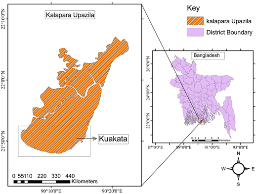
This vast sandy beach has mild slopes toward Bengal Bay and clusters of mangrove plants behindhand that withstand the continual pressures of the tides. A mud flood ridge erected a little hundred meters far away from the shore protects Kuakata’s inner region from tidal waves (Rahman et al., 2013). While much of the terrain inland of the coast is densely forested, the coastline region at Kuakata is immediately exposed to the Bengal Bay. The sand of Kuakata shore is unvarying in the perspective of particle average diameter (d50), which lies midst 0.177 mm to 0.207 mm (Rahman et al., 2013). The shore is comparatively flattering at both the western and eastern ends and the mid portion has come to be steep slope. The coast gradient of Kuakata beach lies from 1:19 to 1:66.
The waves on the coast come from the ocean, and the wave floating phenomenon is of the falling type (Rahman, 1999). The regular waves are quite tiny, during the wet period, the highest waves are around 1.8 m high and in the dry period of January to March, it was very low, and with typical wave heights of about 1 m. Tides in the beach region are semi-diurnal, with daily tide levels ranging from 1 to 1.5 m. During the time of March to October, the wind flows from the south at a mean speed of 3.5 m/s across the Kuakata region. From November through January, the wind moves from the north at a mean speed of 2.6 m/s (Masuma & Tajima, 2011).
3. Data and methods
To carry out this study, multi-temporal Landsat images of Kuakata beach area from seven distinct years, spanning 30 years from 1991 to 2021, were used to detect the shorelines. LANDSAT satellite imageries are created by using MSS, TM, ETM and OLI sensor platforms, gathering various imitated spectral bands of light from the earth items (Chander, Markham, & Helder, 2009). The above-mentioned Landsat imageries were obtained from the website of the United States geological survey (USGS) and include archived LANDSAT images from the National Aeronautics and Space Administration (NASA).
The images were chosen with the data-gathering date in mind. The dry season in Bangladesh, often late winter, is expected to have reduced cloud cover (Table 1), making it ideal for image analysis (Queensland, 2007). Table 1 lists the attributes of satellite images. By using the UTM projection and the WGS 84 datum, all datasets are projected. Figure 2 depicts the DSAS-and RS-based shoreline change flow chart.
Properties of LANDSAT satellite images used in the study
| Date | Sensor | Path/Row | Land cloud cover | Resolution |
|---|---|---|---|---|
| 12/01/2021 | LANDSAT 8 | 137/45 | 0.01 | 30 m |
| 15/01/2016 | LANDSAT 8 | 137/45 | 0.00 | 30 m |
| 17/01/2011 | LANDSAT 5 | 137/45 | 1.00 | 30 m |
| 11/01/2006 | LANDSAT 7 | 137/45 | 1.00 | 30 m |
| 21/01/2001 | LANDSAT 5 | 137/45 | 0.00 | 30 m |
| 09/02/1996 | LANDSAT 5 | 137/45 | 0.00 | 30 m |
| 26/01/1991 | LANDSAT 5 | 137/45 | 0.00 | 30 m |
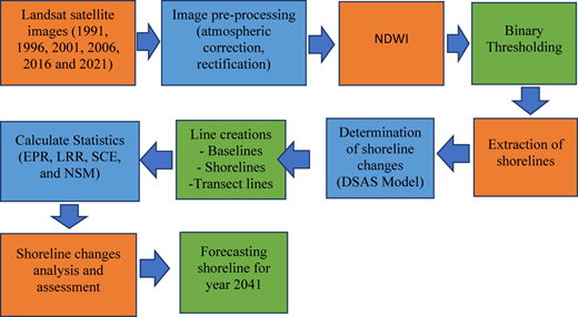
The correctness of the positioning device is allied to the absolute precision of the captured imageries. As, the orbit of satellites is about 500 km above the earth with a speediness of higher than 20,000 km per hr, the positioning of the device essentials to be very sophisticated to be more accurate (Verpoorter, Kutser, Seekell, & Tranvik, 2014). Therefore, in this study, we have used 2 nos. Landsat 8, 1 no. Landsat 7 and 4 nos. Landsat 5 images (Table 1). Comparatively, Landsat 8 images have greater accuracy than the other two, but the Landsat 8 (previously, Landsat Data Continuity Mission (LDCM)) was hurled on an Atlas-V rocket from Vandenberg Air Force Base (VAFB), California on 11 February 2013. As our study area starts from 1991, we had to use other satellite images sacrificing accuracy. On other hand, accuracy also depends on cloud cover. Here most of the images were cloud-free and a maximum of 10% cloud cover is considered here. We have collected the images from the USGS website and their maximum resolution available is 30 m. So technically, we tried to use possible maximum accurate satellite data in this study. The Landsat data, for illustration, has a 30-m resolution, the significance of every pixel standpoint for a 30m × 30m area on the ground. It is contemplated on medium-resolution images, which can cover a full country zone only, however, the level of feature is not well enough to discriminate the separate substances corresponding to households or cars (Data, 2021). Recently, many studies have been conducted using these 30-m resolution images and studies show that these images can detect the rate of change at a wide range. Moreover, we think it is a well-developed procedure that we are using to determine the rate of change in the coastline using 30-m resolution images.
3.1 Correcting the images
The Landsat imageries had pixel values that represented digital numbers (DN), which is an essential radiometric adjustment for improved precision and scientific study (Chander et al., 2009).
Top-of-atmosphere reflectance (or ToA reflectance) is the reflectance which is measured by the space-based sensor flying higher than the atmosphere of the earth. It is used for the reflectance compensates for altered values of the solar irradiance rising from spectral band changes.
Likewise, to compute NDWI, DN must be transformed to the ToA reflectance for improved enactment, as demonstrated in the study of Zhai, Wu, Qin, and Du (2015), Haque and Basak (2017).
Chander et al. (2009) proposed converting DN to Radiance for the Landsat MSS, TM and ETM sensor-derived pictures using the following equations
where is the radiance of spectral unit of “W/(m2 sr. μm),” is the pixel value of quantized calibrated [DN], is the Minimum , is the Maximum , = Minimum scaled to [W/(m2 sr μm)], = Maximum scaled to [W/(m2 sr μm)].
And the following formula is used to convert radiance to ToA reflectance as
where = ToA reflectance [unit less], = 3.14159, is the Earth-Sun distance [astronomical units], is the mean exo-atmospheric solar irradiance [W/(m2 μm)], is the Solar zenith angle [degrees].
For pictures from Landsat OLI, ToA reflectance may be directly translated from DN as U.S. Geological Survey (2016)
where is the reflectance multiplicative scaling factor for the band [unit less], is the reflectance additive scaling factor for the band [unit less].
The values of , , , , , , and are included in a metadata file with the LANDSAT picture. and both are determined using earth sun distance map and mean exo-atmospheric solar irradiance data (Chander et al., 2009). All the imageries utilized were data of Level 1 products, which meant they were ortho-rectified, arithmetically adjusted and co-recorded. The calculation also includes the correction of sun angle.
3.2 Use of spectral index to extract shorelines
As multi-time-based satellite Landsat imageries were employed in this work, an appropriate catalog that employs the band communal in all past and present detectors (i.e. MSS, TM, ETM and OLI) had to be chosen. While both NDWI and NDVI indexes are derived using the satellite image’s Green and Near Infrared bands, common wavelengths are accessible using each Landsat sensor (Khorram, Koch, van der Wiele, & Nelson, 2012). NDWI presented (McFeeters, 1996) is the premium for defining water topographies by means of high accurateness (McFeeters, 2013), and the consequence of the comparison of NDWI. Findings among theoretic and manual attuned thresholds proved to be more precise than the more catalogs stated (Das & Pal, 2016). The following formula is used to compute it:
where is the top atmospheric (ToA) reflectance green band, is top atmospheric (ToA) near-infrared band reflectance.
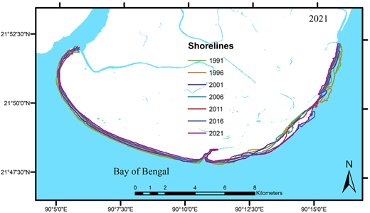
The NDWI usually yields a positive outcome for water features and a negative result for non-water features (McFeeters, 1996). However, it is sight-dependent, and thresholding is required on histogram-based to get of binary image (0 and 1) displaying the water as well as non-water features (Bartuś, 2014). On the NDWI imageries, the binary threshold segmentation approach (Otsu, 1979) was used to discrete land from the water. The threshold was repeatedly computed to split the image into two primary segments: ocean and land. Because the threshold value supplied by Otsu is chosen based on local variables, this segmentation enhanced the accuracy of shoreline extraction (Bouchahma & Yan, 2012). Then after some post-processing, the shorelines were extracted (Bartuś, 2014). Figure 3 shows all seven extracted shorelines for the time scale on the map of 2021.
3.3 Setting the statistical parameters
To calculate change statistics, the DSAS was utilized (Thieler, Himmelstoss, Zichichi, & Ergul, 2009), which can produce SCE considering nine points, NSM, EPR and LRR. Above-mentioned variables are often used in coastline studies, and DSAS can automatically compute them. The EPR method is calculated using the following formula,
where is the distance in meters (m) separating the newest and eldest seashore, is the two coastline locations time interval (yr.).
The LRR technique requires all shoreline locations to be calculated to compute the seashore change rate, which is based on the following linear regression equation:
where is the offset (m) read from the point of reference (baseline), is the cut-off, is the linear regression line slope representing the change rate of shoreline, is the position of shoreline for altered years.
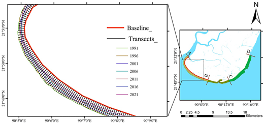
The seven shorelines in the same location from years 1991, 1996, 2001, 2006, 2011, 2016 and 2021 were studied. Transect lines 100 m apart and 1 km long were cast from onshore to seaward from a baseline on the coast (Figure 4). To construct change statistics, the default parameters were +/− 5 m uncertainty and a 95% confidence interval. DSAS creates transect lines that are perpendicular to the baseline and spaced through at a user-specified interval. The rate-of-change data are then calculated using the transect coastline intersections along this baseline (Bouchahma & Yan, 2012).
3.4 Land regression and advancement calculation
A variation in the value of the two binary threshold images was calculated in ArcGIS using the Raster Calculator to estimate the land regression and advancement during three different segments, i.e. 1991–2001, 2001–2011 and 2011–2021. Bouchahma et al. (2012) employed it as a basic yet efficient change detection tool. Polygons were formed by the intersection of two defined shorelines. The region designating erosion and accretion was then manually selected. The pixel counts in the attribute table were translated to km2, and land extraction and land depositing for two separate periods were calculated.
3.5 Forecasting
LRR values were utilized to simulate changes in the coastline near Kuakata by DSAS an ArcGIS extension. Beginning in 1991, this model anticipates the coastline position for each succeeding time step until another shoreline observation is obtained. To enhance the forecast, the model diminishes the difference among the predicted and detected shoreline locations, including adjusting the rate and uncertainty (Basheer Ahammed & Pandey, 2022). The modified shoreline rate change is then used to anticipate further time phases till the next survey date reached, at this point reformed data are sorted out in the model again. By this method, with the derived LLR rate, a crude forecasting of the year 2041 was made.
3.6 The model validation
The remote sensing and geo-statistical models give fascinating insights into the spatial dynamics of coasts (Burgan & Aksoy, 2018). However, there might be significant errors in the concluding results. As a result, model outputs should be validated using observable data. The square root of the variance of the residuals is the root mean square error (RMSE), which represents the absolute fit of the model to the data, i.e. how near the observed data points are to the model’s predicted values (Basheer Ahammed & Pandey, 2022). Lower RMSE values imply better fit, whereas larger values suggest error. As a result, the RMSE was used to validate the actual and forecasted coastline change rates. In this circumstance, the calculated model and satellite-based observations of shoreline deviation rate for 2021 were evaluated using RMSE values.
where xa and ya represent the produced model and xm and ym represent the real x and y positions of the seashore sample points from the reference (baseline). The positional shift in each sample site was obtained by comparing the actual and predicted 2021 coastline.
4. Result and discussion
4.1 The shoreline change envelope (SCE)
SCE denotes the range between nearby and furthest shorelines with relation to the reference point (baseline) which is seen in the timeframe (30 years) research period (1991–2021). Generally, a higher SCE value demonstrates the most active zone of erosion and deposition (Mullick et al., 2020). Figure 5(a) shows the density map and Figure 5(b) shows the line diagram of the observed SCE at Kuakata Coast. The coastline shifting was dominated in CD section with the highest SCE of 722 m and an average shifting of 486 m. Shoreline shifting was also noticeable in segment AB, with an average displacement of 300 m. And the middle part (segment BC), with an average shifting of 190 m, was rather steady. Accordingly, the highest SCE shifting was observed at Red Crab Island east to west bank of Randabad channel. The necessary measures should be taken by the authorities to control the shifting of this mentioned zone.
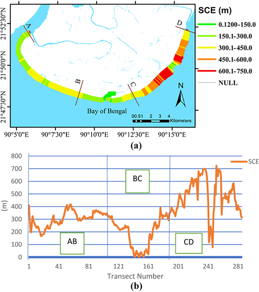
Shoreline change envelope (a) density map (b) line diagram as observed in Kuakata coast
Shoreline change envelope (a) density map (b) line diagram as observed in Kuakata coast
4.2 Net shoreline movement
For each transect, NSM shows the distance between the oldest (in the year 1991) and youngest coastlines (in the year 2021). It denotes a tilt toward either land or water side. Figure 6(a) depicts the density map and Figure 6(b) depicts the line diagram of NSM along the Kuakata Coast, where negative values (−ve) represent landward migration and positive values (+ve) represent seaward movement. In segment CD, north of Dhulaswar Sea Beach has around 580 m landward shifting, whereas the same segment near Red Crab Island shows 620 m seaward shifting. While throughout the AB segment, landward shifting is observed with an average of 257 m. In BC segment, shifting is not so significant.
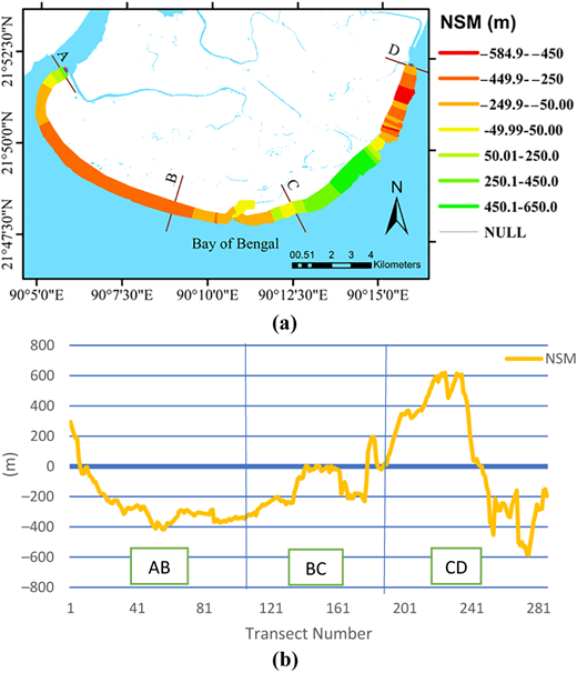
Net shoreline movement (a) density map and (b) line diagram as observed along Kuakata coast
Net shoreline movement (a) density map and (b) line diagram as observed along Kuakata coast
4.3 Regression and advancement of coastal zone
Throughout the study period of 30 years, the quantity of land destruction and development was premeditated for all the sections (segments). The temporal segments were chosen with a 10-year interval. It is apparent after Table 2 that, the total land area of 6.11 square km was gone lost in the Kuakata Coast, while 3.26 square km land area was developed (gained) and overall, the land space was missing by 2.85 square km. The cumulative land gain and loss showed a successive trend of land loss. Land loss in different temporal segments is found to be static in nature. For instance, numerical values of land loss in every segment, i.e. 1991–2001, 2001–2011 and 2011–2021 are around 2 sq. km Figure 7. Whereas the amount of land gain has a rising trend from 1991 to 2021 with numerical values of 0.87 sq. km, 1.01 sq. km and 1.38 sq. km in three consecutive temporal segments (Figure 7) though cumulatively land is lost in every temporal segment (Table 2).
Calculation of the land destruction (loss) and development (gain) for different time period (the *“−ve” sign signifies loss of land)
| Historical segments | Land destruction (sq.km) | Land development (sq.km) | Net destruction/development* (sq.km) | Cumulative destruction/development* (sq.km) |
|---|---|---|---|---|
| 1991–2001 | 2.0 | 0.87 | −1.13 | −1.13 |
| 2001–2011 | 2.05 | 1.01 | −1.04 | −2.17 |
| 2011–2021 | 2.06 | 1.38 | −0.68 | −2.85 |
| 1991–2021 | 6.11 | 3.26 | −2.85 |
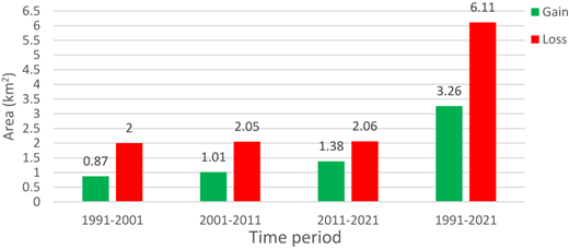
Figure 8 depicts the land loss and gain for segments of all geographical over the various time periods (throughout the whole 30-year timeframe). The AB portion was the most prone to eroding. Almost throughout the whole segment, continuous erosion was observed from 1991 to 2021. Except for some parts of Kuakata National Park, where the land gain is observed from 2011 to 2021. Segment BC also showed continuous erosion from 1991 to 2021. In segment CD, from Red Crab Island to Kuakata National Forrest showed a continuous trend of land gain from 1991 to 2021. But in the north part of the CD segment including Kuakata National Forrest erosion was again dominant and continuous throughout the all-temporal segment (Figure 8).
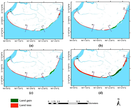
Loss and gain of land scenario in the Kuakata shore from (a) 1991 to 2001, (b) 2001 to 2011, (c) 2011 to 2021 and (d) 1991 to 2021
Loss and gain of land scenario in the Kuakata shore from (a) 1991 to 2001, (b) 2001 to 2011, (c) 2011 to 2021 and (d) 1991 to 2021
From Figure 8, it is evident that the Kuakata Coast is quite predictable in terms of its erosion and deposition characteristics. And overall net erosion with a rate of 0.2 km2/yr. is dominant over net accretion with an average of 0.1 km2/yr. The findings support previous research (Islam, 2013; Rahman et al., 2013) that found the land loss to be more significant than the land gain in this location. According to the study by Islam (2013), in his research, the land loss and land gain rate was shown at 0.29 sq.km/yr. and 0.09 sq.km/yr., respectively, in the Kuakata Coast from 1973 to 2012.
4.4 Rate of shoreline change
The shoreline rate change is one of the most general techniques for coastline experts, engineers and property developers to demonstrate the changing aspects and threats of the coast (Afolabi & Darby, 2022). In this study, we have considered seven shorelines having 5 years’ time intervals from 1991 to 2021 (i.e. 1991–1996, 2001–2006, 2011–2016 and 2016–2021) to determine the change statistics at Kuakata sea beach. For this, we have used two different methods for determining the change rate of shorelines such as LRR and EPR. The benefits of LRR methods are that all shorelines are used, and the method is virginally computational, and the calculation is established on accepted statistical concepts (Himmelstoss, Henderson, Kratzmann, & Farris, 2018). LRR could consider all seven shorelines from 1991 to 2021 (i.e. 1991–1996, 2001–2006, 2011–2016 and 2016–2021). But EPR used only two shorelines: the shorelines of 1991 and 2021. As EPR used only the first and the last shorelines, it was only focused on the initial and final positions of the shoreline. This method (EPR) was not suitable for considering the alternating trend of seaward and landward movement of the line throughout time. However, LRR took six little steps while calculating the change rate from 1991 to 2021. So, it was able to consider those slight alternating variations of shoreline change. As LRR can give more reasonable values than EPR generally. That is why for long-term evaluation LRR was used. LRR showed a more reasonable rate than EPR though with a slight margin. The LRR method is done well than the EPR in the case of the rate of shoreline change premeditated at altered subdivisions (Mullick et al., 2020).
The diverse spatial sections of the coastline (shoreline) have experienced various spatial erraticism during the latter three eras. The variations in temporal and geographical balance were examined to better comprehend the vigorous behavior of the coastline, and the findings are displayed in Figure 9 and Table 3.
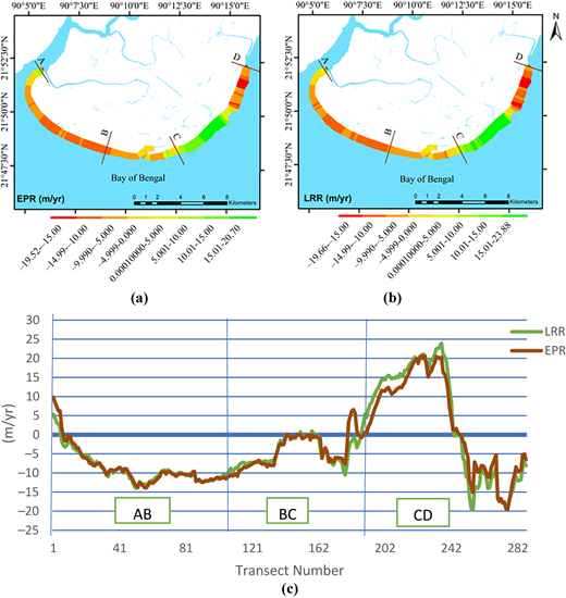
Rate of shoreline change (a) density diagram of EPR (m/yr), (b) density diagram of LRR (m/yr) and (c) variations of EPR and LRR
Rate of shoreline change (a) density diagram of EPR (m/yr), (b) density diagram of LRR (m/yr) and (c) variations of EPR and LRR
Change statistic rate for altered sections of shoreline
| Spatial | EPR | LRR | ||||
|---|---|---|---|---|---|---|
| Segment | Max | Mean | Max | Mean | ||
| Erosion | Accretion | Erosion | Accretion | |||
| AB | −13.94 | 9.78 | −8.59 | −14 | 5.33 | −8.84 |
| BC | −10.85 | 6.55 | −3.99 | −10.55 | 5.39 | −4.21 |
| CD | −19.52 | 20.7 | 3.11 | −19.66 | 23.88 | 3.53 |
| Mean average | −3.15 | −3.17 | ||||
Figure 9(a) depicts a density diagram of a segment-based evaluation of the Kuakata Coast’s shoreline location over the research period as determined using the EPR approach. And Figure 9(b) depicts a segment-based evaluation of the Kuakata Coast’s shoreline location over the research period using the LRR approach. Analyses revealed that the coastline changed at varying rates over the whole research region. In segment CD near Dhulaswar Beach extreme landward movement of shoreline of 19.66 m/year and 19.52 m/year was notable by LRR and EPR, respectively Table 3. Also, the extreme seaward movement was also observed in the same segment near Kuakata National Forrest with a value of 23.88 m/year and 20.7 m/year by LRR and EPR, respectively Table 3. Segment AB experienced landward movement throughout the whole region with a rate of around 8.8 m/year by LRR Table 3. Segment BC was found to be less dynamic than the other two segments. Though it experienced the landward movement of an average of 4.21 m/year with the highest landward movement of 10.5 m/year. The inclusive coastline shifting for the whole study area exhibited negative (landward) movement from the two statistical methods. The mediocre shoreline rate shifting was obtained as −3.15 m/year and −3.17 m/year for EPR and LRR (Table 3).
That means that the whole Kuakata Coast of Bangladesh is shifting landward at a rate of more than 3 meters per year. Segment CD experienced the seaward movement of around 19 m/year, as well as the landward movement of approximately 23 m/year (Table 3). Which is quite less than observed shoreline movement in regions like Patharghata, Galachipa or Barguna Sadar. These regions showed shoreline movement rates higher than 40 m/year (Mullick et al., 2020). As a result, shoreline movement in the research area is considered moderately dynamic. In segment CD the EPR value gave a quite smaller seaward movement of 3.11 m/year (Table 3), whereas LRR gave 3.53 m/year (Table 3). The difference can be due to EPR considering only the 1991 and 2021 shorelines, whereas LRR considered all the seven shorelines as stated by Mullick et al. (2020). According to the study on the shoreline variations in the Vishakhapatnam coastal tract of Andhra Pradesh, India (Baig et al., 2020) that the average shore degradation rate is nearby 1.16 m per year and the rate of aggradation is approximately 1.62 m per year.
The segment AB encounters continual landward movement, making the EPR and LRR approaches suitable for interpreting the pace of shoreline change, with no notable difference between them. The case is like case BC which also observed continuous landward movement in most of its part. Hence, a seashore section that experiences continual landside shifting or seaward movement, the EPR method is moderately agreeable. Likewise, Esmail, Mahmod, and Fath (2019) discovered that the method of the EPR approach performs well at the beaches of current of wave-dominated due to the slow destruction and deposition of the shore. From Figure 9(c), it is evident that in this study region both EPR and LRR showed quite similar results.
Because of their biological importance, coastal wetlands (Rahman et al., 2018) are regarded as important areas. Conversely, the activities of nature and/or humans have a negative impact on certain coastal wetlands. The Kuakata Coast is such a region. The naval and climatic activities intended for coastline erosion as wave, current, surge actions, tidal flood, storm activities, surges of storm and sea level rise are the primary motorists of shoreline modification in that area. The waves of marine, sea currents and tides are the main sources of coastline modification in accordance with the FGD fishermen (Bushra et al., 2021). These consistent spectacles remain the new predominant during the season of monsoon, which reasons loss of land as well as erosion of shoreline. In addition to these natural occurrences, the latest rise in the incidence and severity of beach storms (Bushra, Trepanier, & Rohli, 2019) and tidal floods have expedited the erosional procedure alongside the shore. The forfeiture impacts of frequent sea waves, flows and tides are amplified when these occurrences damage the plant covering, fields of sand dune and sand piles alongside the shore. Because seasonal winds normally sweep from the southwest (Bushra et al., 2021), erosive activities are more prevalent near Kuakata’s west coast. The seashore is mainly receding, nevertheless certain accretionary actions in particular portions of the primarily near Red Crab Island, caused by fluvial and marine processes such as sedimentation, marine action, landform structure and sand agglomeration. These deposits take place due to the low slope and moderate gradient of the central ledge, edifice of polders and embankment at the near side of the seaside boundary. Human accomplishments like land repossession, harbor improvement, etc. along with population concentration are liable for shoreline destruction. Building of bank protection work as embankment and dredging activities in port linking seaways stimulus the river flow rate in current times. The erosion and morphological inequity in the nearby coastline are generated because of dredging actions used for port activities (Dugan et al., 2011). Construction of coastal structures on the seashore distracts the inward surge flux of energy by reflecting waves at diverse shoreline locations. Hence, the degradation procedure grows deeper by shifting its position.
Kuakata was a well-known traveler predicament in a country like Bangladesh; the land restoration has been extravagant for the prior 30 eras and at the early phase there was no one to observe the proceeds of land hand covering for viable motive and digging of sand from the ocean and abolishing of lots of dune fields. These are the conjoint spectacles for the enhancement of a lot of hostels and motels alongside the coast adjacent. Thus, finally consequences in interference with the natural proceeding and hastening of the coast erosion. The deficiency of planning and appropriate laws enactments and legislation for shore management and upkeep are also liable for this beach land ruin. Nonetheless, Bangladesh Government has recently taken several initiatives to retain this famed tourist spot, but the land repossession is still going, and high-rise structures development are ongoing.
4.5 Forecasted shoreline
The shoreline rate change is also one of the furthermost vital factors in the forecast of the future shifting of the oceanfront (Afolabi & Darby, 2022). Henceforward, the rate calculated using the LRR approach was also utilized to provide a rough representation of the coastal position in the year 2041. DSAS tool was used to estimate the future position of shoreline (Himmelstoss et al., 2018). Figure 10(a) shows the position of current and forecasted shoreline position and Figure 10(b) shows the areas of future land loss/gain. The estimated land area loss and gain were calculated using the distance between the existing coastline and the future shoreline position, shown in Table 4.
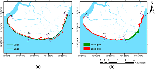
(a) Current and forecasted shoreline position, (b) estimated positions of future land gain/loss
(a) Current and forecasted shoreline position, (b) estimated positions of future land gain/loss
Estimated land loss/gain in forecasted position
| Spatial segment | Land loss (km2) | Land gain (km2) |
|---|---|---|
| AB | 2.229 | 0.0045 |
| BC | 0.816 | 0.015 |
| CD | 1.27 | 2.31 |
| Total | 4.315 | 2.33 |
In total, throughout the study area, 2.33 km2 area will be gained, on the contrary, 4.135 km2 land area will undergo sea. As a result, ultimately around 1.8 km2 land area will be lost (Table 4). The shoreline will continue to move landward in most of the part of Kuakata Coast. Accordingly, the major protecting works ought to be taken by the coast authority on the landward side from future longtime land erosions from the shoreline shifting which will incentive on social life and economic life on the coast side populates. Only near Red Crab Island and some regions, north-east of it will experience seaward movement of shoreline.
4.6 Cross-check
In the current work, the LRR statistical method was used to forecast future coastline location. Shoreline was forecasted for the year 2021 using LRR model based on historical coastline change rates from 1991 to 2016 (1991, 1996, 2001, 2006, 2011 and 2016), and RMSE values were produced by comparing the real shoreline with the forecasted shoreline of the same date. The overall RMS error for the LRR model for the whole anticipated coastline was found to be 83 m in the study, which is a bit high for LRR model. As in a study on the eastern coast of India, LRR model showed RMSE value of 31.17 m and EPR model showed RMSE value of around 80 m (Basheer Ahammed & Pandey, 2022). Since the coastline is vigorous and the positional movement might be variable from time to time, forecasting the shift in the coastline position is extremely difficult. Considering the quite high dynamic nature of the Kuakata shoreline, RMSE of 83 m seems quite reasonable.
5. Conclusion
In this study, RS and GIS were utilized to perform a spatiotemporal analysis of shoreline alteration on the Kuakata Coast and data from the past 30 years (from 1991 to 2021) were evaluated utilizing statistical factors such as LRR and EPR. Land loss and landward movement of shoreline appear to be prevalent along the Kuakata Coast. Both EPR and LRR approach resulted in a landward migration. The average rates are 3.15 m/year and 3.17 m/year, respectively. The study of Baig et al. (2020) revealed the average shore degradation rate is nearly 1.16 m per year and rate of aggradation is approximately 1.62 m per year. Except Red Crab Island and some regions north-east of it, the whole study area experienced land loss, in total 2.85 km2 land loss situation is supportive for submergence of land as the sea level rises along the seaside. This study identifies the locations of the significantly eroded zone in Kuakata from 1991 to 2021. It highlights the places that require special consideration while creating a zoning plan or other structural design. The spatiotemporal shift of coastline will be a potential replacement to assist regional shore planning as a non-structural approach. In the future epoch, the study can be beneficial for taking obligatory activities to develop and endure the sea shoreline to reduce coast zone losses.
Furthermore, the present research will support coastal vulnerability, where shoreline alteration is a crucial physical element. Finally, this study will suggest to the local coastal managers and decision-makers for particularizing the coastal management plans in Kuakata coast zone. We have used LANDSAT satellite imageries which were created using MSS, TM, ETM and OLI sensor stages and gather various imitated spectral bands of light from the earth objects. For more precise, high-resolution altitude imageries alike light detection and ranging (LIDAR) images might be castoff for further study. Also, the effect of land surface temperature (LST) and annual rainfall data can be detected to find if there is any relationship between the factors with erosion and accretion trend in Kuakata Coast region. Besides technical approaches, societal approach like PRA tool which is based on conditions at the indigenous level and different opinions, based on firsthand knowledge, experiences and intergenerational wisdom, can be made use of to better comprehend the shoreline movement trend characteristics.
Funding: There is no funding for this research.
Availability of data and material: On request.
Competing interests: The authors declare that they have no conflict of interest.
Declaration of interest: The authors declare that they have no known competing financial interests or personal relationships that could have appeared to influence the work reported in this paper.

