

The authors derive the necessary mathematics, provide computer simulations, provide links to free and user-friendly computer programs, and analyze real data sets.
Cohen's d, which indexes the difference in means in standard deviation units, is the most popular effect size measure in the social sciences and economics. Not surprisingly, researchers have developed statistical procedures for estimating sample sizes needed to have a desirable probability of rejecting the null hypothesis given assumed values for Cohen's d, or for estimating sample sizes needed to have a desirable probability of obtaining a confidence interval of a specified width. However, for researchers interested in using the sample Cohen's d to estimate the population value, these are insufficient. Therefore, it would be useful to have a procedure for obtaining sample sizes needed to be confident that the sample. Cohen's d to be obtained is close to the population parameter the researcher wishes to estimate, an expansion of the a priori procedure (APP). The authors derive the necessary mathematics, provide computer simulations and links to free and user-friendly computer programs, and analyze real data sets for illustration of our main results.
In this paper, the authors answered the following two questions: The precision question: How close do I want my sample Cohen's d to be to the population value? The confidence question: What probability do I want to have of being within the specified distance?
To the best of the authors’ knowledge, this is the first paper for estimating Cohen's effect size, using the APP method. It is convenient for researchers and practitioners to use the online computing packages.
1. Introduction
Cohen (e.g. 1988) famously argued that researchers should be concerned not only with whether an effect is present but with the size of the effect too. Cohen discussed a variety of different effect size indices, and other researchers have added to the effect size toolbox. Nevertheless, for typical studies, where economic data for two groups are compared, economic data for two countries are compared, or where an experimental group is compared to a control group, Cohen's d remains by far the most popular effect size index. As will be explained in more detail in the subsequent section, Cohen's d denotes the difference in means divided by the standard deviation. Thus, Cohen's d provides valuable information about how much the means differ in standard deviation units.
One reason that scientists in the social and economic sciences have found Cohen's d useful is that many of the dependent measures these sciences do not have intrinsic meaning. For instance, whereas it might be reasonably clear what a dollar means, the meaning of a unit on an attitude scale might be less clear. If the mean attitude in the experimental condition is 2 and the mean attitude in the control condition is 1, is this a small difference or a large one? By converting the difference in means to Cohen's d, the researcher can gain an idea of the size of the difference in standard deviation units, even when the scale units are not themselves intrinsically meaningful. Another advantage of Cohen's d is that it facilitates comparisons across studies. Even if scale units are different for different studies, thereby rendering them seemingly impossible to compare, researchers still can compare in terms of standard deviation units. Many researchers have taken advantage of this, particularly in meta-analytic research. Despite the popularity of Cohen's d and its obvious usefulness, there remains an important limitation. Specifically, the Cohen's d that a researcher obtains in a particular experiment is a sample statistic. It is not a population value. Typically, researchers are not interested in sample statistics for their own sake, but because they provide useful estimates of population values. Thus, there is an important question that has not been properly addressed: how well does Cohen's d estimate the population effect size? Although researchers have long known how to compute traditional confidence intervals for Cohen's d, traditional confidence intervals do not properly address the question. This is because, for example, although 95% of 95% confidence intervals surround the population parameter, it is not the case that the population parameter has a 95% chance of being within a 95% confidence interval. This last is unknown. In addition, Trafimow and Uhalt (2020) have shown that sample confidence intervals tend to be inaccurate representations of population confidence intervals unless sample sizes are much larger than those typically employed. An alternative way to address the issue is to use the a priori procedure (APP) that has been employed previously in a variety of ways not pertaining to Cohen's d (e.g. Li et al., 2020; Trafimow, 2017, 2019; Trafimow and MacDonald, 2017; Trafimow et al., 2020a; Wang et al., 2020, 2021; Wei et al., 2020). Although the APP uses confidence intervals, it does so in a way that deviates importantly from traditional confidence intervals. To use APP thinking to address Cohen's d, the researcher would ask the two bullet-pointed questions below.
The precision question: How close do I want my sample Cohen's d to be to the population value?
The confidence question: What probability do I want to have of being within the specified distance?
For example, the research might wish to have a 95% probability of obtaining Cohen's d within a tenth of a standard deviation of the population value. The present goal is to determine the sample size the researcher needs to collect to meet the precision and confidence specifications in the contexts of independent and matched samples experimental designs.
This paper is organized as follows. Definitions of Cohen's effect sizes for both populations and samples are given in Section 2, together with properties of noncentral t distributions. In Section 3, the APP methods are applied for estimating population effect size θ in independent case and θD in dependent case. In Section 4, the simulation study, the coverage rate, and real data examples are provided in supporting our main results given in Section 3. Conclusion remarks are given in Sections 5.
2. Preliminaries
Effect size is a statistical concept that measures the strength of the relationship between two variables on a numeric scale. For example, in medical education research studies that compare different educational interventions, effect size is the magnitude of the difference between groups. The absolute effect size is the difference between the average, or mean, outcomes in two different intervention groups. The standard deviation of the effect size is of critical importance, since it indicates how much uncertainty is included in the measurement. For more details and applications, see, Sullivan and Feinn (2012), Schafer and Schwarz (2019), Bhandari (2020).
Cohen's d is one of the most common ways to measure effect size, which is known as the difference of two population means and it is divided by the standard deviation from the data. Mathematically, Cohen's effect size is denoted by:
where μ1 and μ2 are means of two populations, and σ is the standard deviation based on either or both populations.
Cohen's d is defined as the difference between two means divided by a standard deviation for the data obtained from both populations:
where and are sample means and S, defined by Jacob Cohen, is the pooled standard deviation (for two independent samples)
and n1, S1, n2, S2 are sample sizes and sample variances of two independent samples, respectively.
Note that confidence intervals of standardized effect sizes, especially Cohen's d, rely on the calculation of confidence intervals of noncentrality parameters. In order to find the minimum sample sizes for estimating the Cohen's effect size θ given in (2.1) by Cohen's d given in (2.2), we need the following definition.
Let Z and U be independent random variables, Z ∼ N(λ, 1), the normal distribution with mean λ and standard deviation 1, and , the chi-square distribution with m degrees of freedom. The random variable T given by
It is easy to obtain the following properties of T ∼ tm(λ) (see Nguyen and Wang, 2008).
The probability density function (pdf) of T is given by
The mean and variance of T are
and
respectively. For convenience, if we use the correction factor J(m) given by
then the mean and the variance of T are
and
We will use the following results in the proofs of our main results to be given in next section.
Proof. From the basic statistics, we know that.
so that .
and so that as and are independent.
Now by Definition 2.1, , the desired result follows. □
For the dependent case, we have the following result.
Let be a random sample of size n from a bivariate normal population with mean vector μ and covariance matrix Σ, where
Let Di = X1i − X2i, i = 1, …, n and and be the Cohen's sizes of the population and matched sample, respectively, where
Proof. Note that so that , where . Also it is easy to know that
and and are independent. Therefore, by Definition 2.1,
so that the desired result follows. □
The graphs of density curves of tm(λ) with different mean values J(m)λ and different degrees of freedom m are given in Figures 1 and 2, respectively. From graphs, we know that (i) density curves are symmetric about mean J(m)λ, which is a function of m, so that the equal tailed confidence intervals should be the best choice, and (ii) density curves tend to N(λ, 1) as m to ∞.
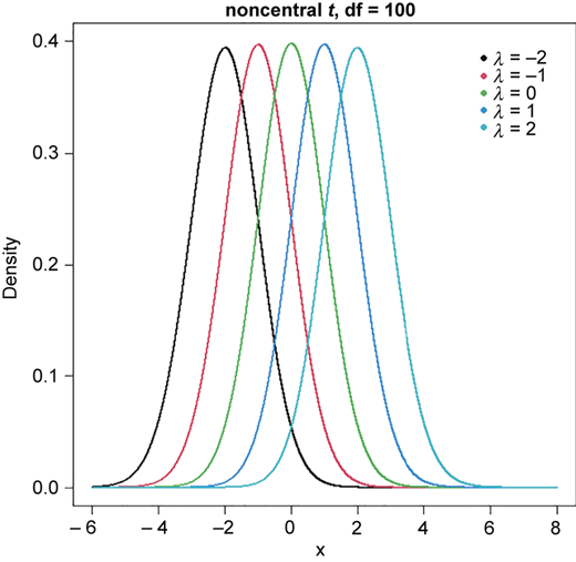
The density curve of noncentral t-distribution with degrees of freedom 100 and different values of noncentral parameter λ
The density curve of noncentral t-distribution with degrees of freedom 100 and different values of noncentral parameter λ
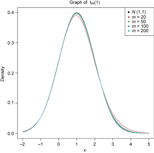
The density curve of noncentral t-distribution with noncentral parameter λ = 1 and different values of degrees of freedom
The density curve of noncentral t-distribution with noncentral parameter λ = 1 and different values of degrees of freedom
For a given the confidence level c = 1 − α, the c 100% confidence intervals of λ based on T1 with m1 degrees of freedom and T2 with m2 with m1 < m2 degrees of freedom have the following relationship:
3. The APP methods for estimating both θ and θD
In this section, we will apply the APP methods for estimating Cohen's effect size θ in independent samples' case and θD in matched sample case.
3.1 The minimum sample size required for estimating θ
First, we consider two independent samples from two normal populations and with equal unknown variances: .
Let be a random sample of size n1 from N(μ1, σ2), be a random sample of size n2 from N(μ2, σ2). Assume that two samples are independent. Let c be the confidence level and f be the precision which satisfies
J(n1 + n2 − 2) is the correction factor given in (2.4). Both θ and d are given in (2.1) and (2.2). Let n = min{n1, n2} and fT(⋅) be the density of t-distribution with degrees of freedom 2(n − 1) and noncentrality parameter . Then the required sample size n can be obtained by solving
Proof. By Proposition 2.1, we know that , where . Thus, the mean and variance of d, are given, respectively, by
and
Now it is easy to obtain the density of , which is symmetric about 0 and given by
where is the density of T1. Note that if we have two independent random samples of sizes n1 and n2, we can construct the 100c% confidence interval for θ based on (3.7). Now, let , which has a noncentral t distribution with n1 + n2 − 2 degrees of freedom and noncentrality parameter . Thus, the unbiased estimator of θ is . Note that the variance of d1 is
Therefore, we can setup the confidence interval for given confidence level c and precision f, which is given in (3.1). Since there are two unknowns n1 and n2, there are no solutions using Equation (3.1) so we need to modify this equation. Let n = min{n1, n2} so that the degrees of freedom n1 + n2 − 2 ≥ 2n − 2. Suppose that we have two independent samples of size n in both; then, , and the distribution of is the noncentral t with 2(n − 1) degrees of freedom and the noncentrality parameter so that its mean and variance are
Thus, the standardized random variable has the density given in Equation (3.3). Therefore, the required n can be obtained by solving Equation (3.2). Similarly to Remark 2.2, we know that , where Hm,(1−c)/2 is the critical value of the distribution H. It is easy to see that
so that the desired results follows. □
The required n obtained in Theorem 3.1 is unique. Also, if the conditions in Theorem 3.1 are satisfied, we can construct a c × 100% confidence interval for
In order to see that Equation (3.9) holds numerically, we provide probabilities of the c = 95% confidence intervals for different sample sizes n1 and n2, which is given in Table 1.
Probabilities of the c = 95% confidence intervals for different sample sizes n1 and n2
| θ | n1 | n2 | df | H2n−2,(1−c)/2 | P(|H| < H2n−2,(1−c)/2) |
|---|---|---|---|---|---|
| 0 | 100 | 100 | 198 | 13.87366 | 0.95 |
| 120 | 218 | 0.9395 | |||
| 150 | 248 | 0.9267 | |||
| 0.2 | 100 | 100 | 198 | 13.87366 | 0.9512 |
| 120 | 218 | 0.9408 | |||
| 150 | 248 | 0.9281 | |||
| 0.5 | 100 | 100 | 198 | 14.04887 | 0.9528 |
| 120 | 218 | 0.9427 | |||
| 150 | 248 | 0.9302 | |||
| 0.8 | 100 | 100 | 198 | 14.14443 | 0.9547 |
| 120 | 218 | 0.9445 | |||
| 150 | 248 | 0.9322 |
Researchers can access at the following website https://appcohensd.shinyapps.io/independent/ to obtain the required sample size. The input variables are the value of θ0 from the previous data by previous data or θ0 = 0, precision f, and confidence level c. For convenience, the output variable is the required sample size n = min{n1, n2}. The required sample sizes for different values of precision f = 0.1, 0.15, 0.2, 0.25, confidence levels c = 0.95, 0.90 and θ0 = 0, 0.1, …, 1 for independent case are given in Table 2. The relationship between required sample n and parameter θ for different values of precision f is given in Figure 3.
The desired sample sizes n for f = 0.1, 0.15, 0.2, 0.25, θ = 0, 0.1, …, 1 and c = 0.95, 0.9 in the independent case
| θ | 0 | 0.1 | 0.2 | 0.3 | 0.4 | 0.5 | 0.6 | 0.7 | 0.8 | 0.9 | 1 | |
|---|---|---|---|---|---|---|---|---|---|---|---|---|
| f = 0.1 | c = 0.95 | 382 | 384 | 386 | 389 | 392 | 396 | 405 | 411 | 415 | 423 | 436 |
| c = 0.90 | 268 | 269 | 271 | 273 | 276 | 279 | 283 | 287 | 294 | 300 | 304 | |
| f = 0.15 | c = 0.95 | 169 | 170 | 171 | 173 | 174 | 176 | 180 | 183 | 186 | 191 | 194 |
| c = 0.90 | 118 | 119 | 120 | 121 | 122 | 124 | 125 | 127 | 130 | 133 | 135 | |
| f = 0.2 | c = 0.95 | 94 | 95 | 96 | 97 | 98 | 99 | 100 | 102 | 104 | 106 | 110 |
| c = 0.90 | 66 | 66 | 67 | 67 | 68 | 69 | 70 | 71 | 73 | 74 | 76 | |
| f = 0.25 | c = 0.95 | 60 | 60 | 61 | 62 | 63 | 63 | 64 | 65 | 67 | 68 | 70 |
| c = 0.90 | 41 | 41 | 42 | 42 | 43 | 44 | 44 | 45 | 46 | 47 | 49 | |
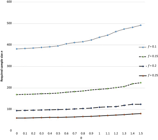
The relationship between required sample n and parameter θ for c = 0.90 and different values of precision f
The relationship between required sample n and parameter θ for c = 0.90 and different values of precision f
3.2 The minimum sample size of Cohen's d needed for a given sampling precision in matched samples
Let be a random sample of size n from a bivariate normal population with mean vector μ and covariance matrix Σ, where
Denote Di = X1i − X2i, i = 1, …, n. Let and be the Cohen's effect sizes of the population and matched sample, respectively, where
Let c be the confidence level and f be the precision which satisfies
Then the required sample size n can be obtained by
Proof. By Proposition 2.2, we know that , where .
It is easy to see that the mean and variance of dD are given by
Thus, the density of H is given in Equation (3.13). Now, we know that , where . Then, the variance of is
From the distribution of H, we can obtain the required sample size n which is given in Equations (3.12) - (3.14) so that the desired result follows. □
The value of n obtained is unique with f. Also, if the conditions in Theorem 3.2 are satisfied, we can construct a c × 100% confidence interval for θD given by
Researchers can access at the following website: https://appcohensd.shinyapps.io/matched/
The input variables are the confidence level c, precision f, correlation coefficient ρ and obtained from previous data information. The default value of θD = 0. The output is the desired sample size n required. Table 3 provides the n for c = 0.90, 0.95 for different values of f and different values of 's. Also the relationship between n and θD is given in Figure 4.
The desired sample sizes n for f = 0.1, 0.15, 0.25, θD = 0, 0.2, 0.5, 0.8 and c = 0.95, 0.9 in the case of ρ = 0.2, 0.5, 0.8
| θD | 0 | 0.2 | 0.5 | 0.8 | ||
|---|---|---|---|---|---|---|
| f = 0.1 | ρ = 0.2 | c = 0.95 | 382 | 389 | 418 | 470 |
| c = 0.90 | 267 | 273 | 293 | 330 | ||
| ρ = 0.5 | c = 0.95 | 382 | 392 | 436 | 517 | |
| c = 0.90 | 267 | 276 | 304 | 363 | ||
| ρ = 0.8 | c = 0.95 | 382 | 407 | 514 | 705 | |
| c = 0.90 | 267 | 284 | 361 | 490 | ||
| f = 0.15 | ρ = 0.2 | c = 0.95 | 168 | 173 | 186 | 207 |
| c = 0.90 | 117 | 120 | 130 | 144 | ||
| ρ = 0.5 | c = 0.95 | 168 | 175 | 198 | 231 | |
| c = 0.90 | 117 | 122 | 135 | 163 | ||
| ρ = 0.8 | c = 0.95 | 168 | 180 | 234 | 325 | |
| c = 0.90 | 117 | 126 | 162 | 216 | ||
| f = 0.25 | ρ = 0.2 | c = 0.95 | 59 | 61 | 67 | 76 |
| c = 0.90 | 40 | 42 | 46 | 51 | ||
| ρ = 0.5 | c = 0.95 | 59 | 62 | 71 | 81 | |
| c = 0.90 | 40 | 42 | 48 | 58 | ||
| ρ = 0.8 | c = 0.95 | 59 | 65 | 82 | 118 | |
| c = 0.90 | 40 | 44 | 58 | 77 | ||
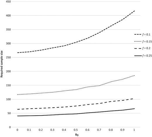
The relationship between required sample n and parameter θD for ρ = 0.5, c = 0.90 and different values of precision f
The relationship between required sample n and parameter θD for ρ = 0.5, c = 0.90 and different values of precision f
4. Simulation and real data examples
In this section we will provide some simulation results and two real data examples to support our main results. Based on M = 100,000 runs, coverage rates of the confidence intervals and the corresponding point estimates of θ in independent case and θD for matched data are given in Tables 4 and 5. From these two tables, we can see that the performances of our APP procedures work very well and the biases are really small.
The corresponding point estimates of θ and the coverage rates when n satisfies the required minimum sample size for f = 0.1, 0.15, 0.2, 0.25, θ = 0, 0.2, 0.5, 0.7, 1 and c = 0.95, 0.9 in the independent case
| f | θ | c = 0.95 | c = 0.90 | ||||
|---|---|---|---|---|---|---|---|
| n | Coverage rate | n | Coverage rate | ||||
| 0.1 | 0 | 382 | 0.0001 | 0.9489 | 268 | 0.0001 | 0.8971 |
| 0.2 | 386 | 0.1999 | 0.9509 | 271 | 0.2004 | 0.8976 | |
| 0.5 | 396 | 0.5002 | 0.9499 | 279 | 0.5007 | 0.8988 | |
| 0.7 | 411 | 0.7007 | 0.9509 | 287 | 0.7012 | 0.9008 | |
| 1 | 436 | 1.0007 | 0.9509 | 304 | 1.0012 | 0.8997 | |
| 0.15 | 0 | 169 | −0.0002 | 0.9489 | 118 | −0.0003 | 0.8976 |
| 0.2 | 171 | 0.2008 | 0.9499 | 120 | 0.2006 | 0.8998 | |
| 0.5 | 176 | 0.5007 | 0.9503 | 124 | 0.5009 | 0.9006 | |
| 0.7 | 183 | 0.7013 | 0.9511 | 127 | 0.7023 | 0.9011 | |
| 1 | 194 | 1.0019 | 0.9508 | 135 | 1.0031 | 0.8987 | |
| 0.2 | 0 | 94 | −0.0004 | 0.9473 | 66 | 0.0005 | 0.8981 |
| 0.2 | 96 | 0.2013 | 0.948 | 67 | 0.1998 | 0.8978 | |
| 0.5 | 99 | 0.5009 | 0.9497 | 69 | 0.5045 | 0.898 | |
| 0.7 | 102 | 0.7023 | 0.952 | 71 | 0.7029 | 0.8985 | |
| 1 | 110 | 1.0025 | 0.9469 | 76 | 1.0051 | 0.9007 | |
| 0.25 | 0 | 60 | 0.0002 | 0.9469 | 41 | −0.0005 | 0.8913 |
| 0.2 | 61 | 0.2009 | 0.9472 | 42 | 0.2026 | 0.8951 | |
| 0.5 | 63 | 0.5028 | 0.9469 | 44 | 0.5049 | 0.898 | |
| 0.7 | 65 | 0.7046 | 0.9489 | 45 | 0.7058 | 0.8974 | |
| 1 | 70 | 1.0054 | 0.9522 | 48 | 1.0085 | 0.8983 | |
The corresponding point estimates of θD and the coverage rates when n satisfies the required minimum sample size for f = 0.1, 0.15, 0.2, 0.25, θ = 0, 0.2, 0.5, 0.7, 1, ρ = 0.2, 0.5, 0.8 and c = 0.95 in the matched case
| f | θD | c = 0.95, ρ = 0.2 | c = 0.95, ρ = 0.5 | c = 0.95, ρ = 0.8 | ||||||
|---|---|---|---|---|---|---|---|---|---|---|
| n | Coverage rate | n | Coverage rate | n | Coverage rate | |||||
| 0.1 | 0 | 382 | 0.0001 | 0.9503 | 382 | −0.0001 | 0.9488 | 382 | 0.0001 | 0.9499 |
| 0.2 | 389 | 0.2002 | 0.9496 | 392 | 0.2004 | 0.9502 | 407 | 0.2006 | 0.9501 | |
| 0.5 | 418 | 0.5007 | 0.9514 | 436 | 0.5007 | 0.9505 | 514 | 0.5008 | 0.9535 | |
| 0.7 | 447 | 0.7008 | 0.9506 | 493 | 0.7011 | 0.9529 | 625 | 0.7009 | 0.9513 | |
| 1 | 514 | 1.0015 | 0.9517 | 594 | 1.0011 | 0.9539 | 892 | 1.0008 | 0.9542 | |
| 0.15 | 0 | 168 | −0.0003 | 0.9468 | 168 | −0.0001 | 0.947 | 168 | −0.0001 | 0.9486 |
| 0.2 | 173 | 0.2013 | 0.9499 | 175 | 0.2009 | 0.9495 | 173 | 0.2007 | 0.9509 | |
| 0.5 | 186 | 0.5024 | 0.9498 | 198 | 0.5019 | 0.9529 | 207 | 0.5014 | 0.9544 | |
| 0.7 | 199 | 0.7027 | 0.9515 | 222 | 0.7024 | 0.9544 | 291 | 0.7019 | 0.9564 | |
| 1 | 234 | 1.0033 | 0.9545 | 257 | 1.0032 | 0.9509 | 391 | 1.0018 | 0.9517 | |
| 0.2 | 0 | 93 | 0.0001 | 0.9448 | 93 | −0.0003 | 0.9444 | 93 | 0 | 0.9452 |
| 0.2 | 97 | 0.2016 | 0.9486 | 98 | 0.2013 | 0.949 | 102 | 0.2014 | 0.9511 | |
| 0.5 | 104 | 0.5038 | 0.9485 | 110 | 0.5039 | 0.9509 | 129 | 0.5026 | 0.9524 | |
| 0.7 | 115 | 0.704 | 0.9546 | 125 | 0.7043 | 0.9531 | 159 | 0.7034 | 0.9513 | |
| 1 | 129 | 1.0058 | 0.9527 | 154 | 1.0044 | 0.9575 | 228 | 1.0034 | 0.956 | |
| 0.25 | 0 | 59 | 0.0001 | 0.9448 | 59 | 0.0001 | 0.9451 | 59 | −0.0003 | 0.9438 |
| 0.2 | 61 | 0.2025 | 0.9486 | 62 | 0.2022 | 0.9489 | 65 | 0.2019 | 0.9491 | |
| 0.5 | 67 | 0.5062 | 0.9497 | 71 | 0.5057 | 0.9514 | 82 | 0.5042 | 0.9532 | |
| 0.7 | 73 | 0.7071 | 0.9526 | 80 | 0.7066 | 0.9538 | 105 | 0.7051 | 0.9562 | |
| 1 | 82 | 1.0098 | 0.9529 | 97 | 1.0075 | 0.9563 | 146 | 1.0055 | 0.956 | |
To evaluate our results, we provide a real data example for independent and match sample cases, respectively.
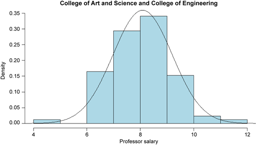
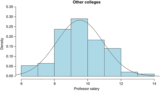
Consider the salary data (in 2011) of all professors from College of Arts and Sciences and College of Engineering (population 1 with size 85) and other colleges (population 2 with size 93) of New Mexico State University, which are publicly available https://riograndefoundation.org/downloads/rgf_pr_nmsu.pdf
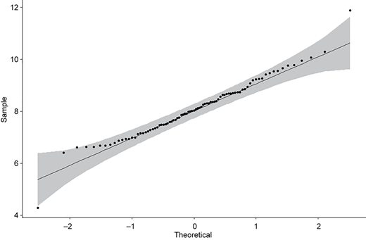
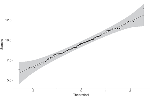
The estimated distributions based on the data set are approximately N(8.0868, 1.10992) for population 1 and N(9.5273, 1.41152) for population 2 (with unit $10,000) (see Figures 5 and 7). The Q–Q plots of the data sets are given in Figures 6 and 8, showing that the scatters lie close to the line with no obvious pattern coming away from the line in both Q–Q plots. Now we consider the 95% confidence interval of θ with precision f = 0.25 and default θ = 0. From Table 2, the minimum sample sizes n needed is 60, so we randomly choose samples of size 60 from both populations and obtain the value of Cohen's d is d = −1.1430. Then by Remark 3.1, the 95% confidence interval of θ is [−1.4900, −0.7814], which includes the true value of population effect size θ = −1.1284.
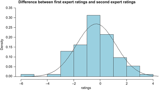
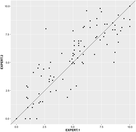
For matched case, we consider the data set named “Rugby” from Pakage “PairedDate” in R by Champely (2018). This data set provides the ratings on a continuous ten-point scale of two experts about 93 actions during several rugby union matches. Let D be the difference between ratings of two experts. The histogram and estimated density curve of D are given in Figure 9. From the data, we obtain and SD = 1.4872. The pattern of the points of the scatter plot shown in Figure 10 shows a positive linear relationship between this two variables. After calculation, we get the correlation coefficient is ρ = 0.85. Now we consider the 95% confidence interval of population effect size θD with precision f = 0.25 and default θ = 0. By the shinyApp provided in Section 4 for matched data, the minimum sample sizes n needed is 59. Randomly select a sample with 59 paired data; then by Remark 3.2, we have the 95% confidence interval of θD is [−0.3122, −0.0371], which includes the true value of population effect size −0.1122.
5. Conclusion remarks
Our goal was to derive ways to perform the APP with respect to Cohen's d for independent and matched samples. The present mathematics provide those derivations. In turn, computer simulations support the mathematical derivations. We also provide links to free and user-friendly programs to facilitate researchers performing the APP to determine sample sizes to meet their specifications for precision and confidence. An advantage of the programs is that even researchers who are unsophisticated in mathematics nevertheless can avail themselves of APP advantages.
In addition to the obvious benefit of aiding researchers who wish to compute Cohen's d determine the samples sizes they need the present mathematics provide an additional benefit. Specifically, the famous article in Science by the Open Science Collaboratio (2015) included replications of studies in top psychology journals. They found that the average effect size in the replication cohort of studies was less than half that in original cohort of studies. Thus, effect sizes tend not to replicate across study cohorts. Our suspicion is that one reason for irreproducibility is that sample sizes are too small and traditional power analyses are insufficient because they do not address the precision issue (Trafimow and Myüz, 2019; Trafimow et al., 2020b), though significance testing doubtless plays a role too. The present mathematics, along with the links to computer programs, provide a solution. We hope and expect that researchers who wish to use Cohen's d to index their effect sizes will be better able to determine appropriate sample sizes, and thereby increase reproducibility in the social sciences.
