

In this research, the main purpose is to use a suitable structure to predict the trading signals of the stock market with high accuracy. For this purpose, two models for the analysis of technical adaptation were used in this study.
It can be seen that support vector machine (SVM) is used with particle swarm optimization (PSO) where PSO is used as a fast and accurate classification to search the problem-solving space and finally the results are compared with the neural network performance.
Based on the result, the authors can say that both new models are trustworthy in 6 days, however, SVM-PSO is better than basic research. The hit rate of SVM-PSO is 77.5%, but the hit rate of neural networks (basic research) is 74.2.
In this research, two approaches (raw-based and signal-based) have been developed to generate input data for the model: raw-based and signal-based. For comparison, the hit rate is considered the percentage of correct predictions for 16 days.
1. Introduction
Because of the many turnovers that can be achieved by the prediction of stock price, it has been a topic of thought and discussion among investors and scientists. In order to have a precise prediction, correct information on the stock market, its changes and trend forecasting, a result of the close to random-walk behavior of a stock time series is required. Due to nonlinear stock market fluctuation stock price prediction is complicated and in order to tackle this investors and financial analysts need reliable tools (Jasemi et al., 2011a, b).
With the help of A.I this issue is approximately addressed since they can understand nonlinear relations and are able to apply the dominant uncertainty in the stock market.
With the advances that have happened through A.I, more accurate new prediction methods than traditional ones have been realized. Nevertheless, each of the new methods is not exempt from disadvantages. They are classified into two categories, which are: fundamental and technical analyses. The fundamental analysis investigates various factors with great impact on the stock market such as micro-economics, macro-economics, politics and even psychology, however, most of the time knowledge is not available yet.
The technical analysis makes procrastinations regarding the previous patterns, despite the fact that because of the noise, these patterns are not always easily notices.
(Xiao et al., 2012). Improvements in the digital era have made predictions also a technological matter. The most promising techniques now are based on artificial neural networks (ANNs), and recurrent neural networks, which are basically involved in machine learning; these are the most commonly used approaches (Liu et al., 2020).
In a lot of real cases, one of the most difficult problems is raining a deep neural network that can generalize well to new data. Other solutions like early stopping or cross-validation (regularization) or Bayesian methods have been developed to overcome this issue (Mackay, 1992).
Support vector machine (SVM) is a recently innovated method that is listed as supervised learning and successfully tackles limitations. Classification and regression are the two applications of this method. With the help of SVM, global optimal solutions can be found, which is not the case in ANN which frequently yields local optimal solutions. In this procedure, a single data component is plotted as a point in n-dimensional space (n is the number of accessible highlights of the dataset) in which the esteem of highlight is the esteem of a specific facility. Through identification of the hyperplane parting the two classes, classification is done; thus, the accuracy of backup vectors is dependent on the setting up of the parameters. The tendency of investors to use machine learning algorithms like Japanese candlestick forecasting models in the stock market stems from the above-mentioned merits of it such as optimization methods. As an example (Jasemi et al., 2011a, b), use a supervised feed-forward neural network (Barak et al., 2015), applies a Wrapper Adaptive Neuro-Fuzzy Inference system-Independent Component Analysis (ANFIS-ICA) as a fuzzy neural network; and (Ahmadi et al., 2016) use a Nonlinear Autoregressive Exogenous (NARX) as a nondynamic neural network as an analyst for their candlestick models. In previously mentioned studies, computational intelligence methods for stock price forecasting were used; and for the sake of finding the proper number of variables, meta-heuristic algorithms were applied.
Among them, in spite of the fact that the prevalence of Molecule Particle swarm optimization (PSO) is demonstrated in numerous studies, in times cases, it was used to solve prediction models.
In some optimization algorithms, an optimizer is used. Although, making alterations towards “local” and “global” best particles, is nearly similar to the crossover operation used by genetic algorithms as well (Mahmoudi et al., 2020). It can be seen that the fitness function is in PSO that measures the closeness of the corresponding ways to the optimum.
What actually differentiates the PSO and the evolutionary computing?
The biggest difference between the PSO concept and evolutionary computing is flying potential ways through hyperspace is accelerating toward “better” solutions, while evolutionary computation schemes operate directly on potential solutions that are explained as locations in hyperspace (Kennedy, 2011).
As there is not enough literature done in this area, in this study hybrid SVM along with two meta-heuristic algorithms the objective of this study is movement prediction of movement stock prices with a direct effect on the combination of input variables and examining the precision of such forecasts (Ahmadi et al., 2018). To optimize the model and parameters two meta-heuristic algorithms which are PSO and neural network are used.
PSO has been used for many real-world engineering cases, especially structural engineering problems. PSO has the following advantages over other popular hyperparameter optimization methods like grid search or Bayesian optimization: Simple concept, easily programmable, faster in convergence and mostly provides better solution. PSO is based on random element and the cost of error.
Additionally, for having the best SVM parameters different algorithms are applied. We choose to develop the SVM parameters through PSO algorithms, to prepare a comparative analysis of the performance of two metaheuristic algorithms. According to the recorded literature in seldom of the relative researches, this survey has been taken into consideration.
This research contributes to the below points:
New machine learning methods are introduced and used to achieve the most suitable SVM parameters
A thorough analysis of candlestick coefficients in order to select the optimized signal forecast approach
Application of PSO-SVM model in two different periods to analyze the model's performance
This research is explained as follows:
The literature review is written in the second section. In the third section, backgrounds and last studies are introduced, which is a basis for a better understanding of the nature of this work. A new model of the study as well as the conceptual basics of the models is explained in section 4. Section 5 runs the model with real data and presents the results. Section 6 explains how our model is valid and the final discussions of the study, conclusion and references are covered in sections 7 and 8.
2. Literature review
The previous research processes of the researchers and financial investors have indicated how much the stock market and the efficient factors severely influence countries forming economic structures. So far, these factors as variables have predicted the influential factors for determining price in a market. In this regard, many techniques and frameworks have been presented so far that have been investigated in this part in three sections technical analysis, fundamental analysis and combined analysis. Moreover, each analysis has been developed through various dimensions such as machine learning models, data sources' nature, accuracy and error criteria, and modeling by heuristic or metaheuristic methods.
In predictive models of financial variables that have been done based on technical methods, it is assumed that prices change in the stock market can be predicted based on the previous prices. In this approach, the analysts believe that all the influential factors are considered in the market prices. In addition, they claimed that it is unnecessary to pay attention to factors such as the expected efficiency time of investment and the natural stock value that is mostly predicted in structural methods (Singh, 2022) precisely. The experts' opinion determines prediction rules among all the technical indexes, including the moving average (MA), moving average convergence/divergence (MACD), the Aroon indicator and money flow index that these rules are usually fixed and do not change (Rouf et al., 2021). In order to compensate for the shortcomings of each method (technical and fundamental), most researchers have developed machine learning methods that are classified as modern methods for predicting stock moves. These methods increase prediction accuracy to a great extent than the traditional methods (Ballings et al., 2015). Furtherly, according to heterogeneous data and complex stock prices, they can earn appropriate patterns for prediction. These methods have been applied in two sets of linear and nonlinear methods (Selvin et al., 2017). For example. The other researcher (Cao, 2021) used linear regression, Least Absolute Shrinkage and Selection Operator (LASSO), regression trees, bagging, random forest and boosted tress to analyze data and predict the stock price movement of 35 companies on the New York stock exchange. Simultaneously with the development of artificial intelligence methods, nonlinear methods of machine learning have been proposed.
Heuristics and metaheuristic algorithms play an important role in these methods, and their extensive use in recent years indicates how successful they have been. Another study (Shen et al., 2020) has highlighted that using methods of ANNs and SVM can simply find the hidden framework in the prediction via the self-learning process. The SVM methods are introduced in the framework of generalized portrait methods. They are a kind of computer learning that have successfully performed in diagnosing pattern because stock market systems have nonlinear nature (Vapnik and Chervonenkis, 2013). These methods accurately predict the relationship between the input and output data by combining heuristic and technical methods. For example (Selvin et al., 2017), conducted a comparative analysis of price collection of the companies' stock in the National Stock Exchange (NSE) list that reports excellence of deep learning methods. They have used the sliding window method for overlapping data in their study. In addition (Abinaya et al., 2016), have analyzed the stock price of 29 companies in the NITFY 50 (Indian stock market index) list to investigate the dependence between stock price and its size and to check the function of the deep learning method in the correct prediction of stock price. Goel et al. (2019) also used a combination of linear regression and Long short-term memory (LSTM) for prediction (Ananthi and Vijayakumar, 2021) applied the candlestick chart and regression to predict the model.
Wang et al. (2003) use SVM to foresee air quality, in which the efficiency of neural networks based on the radius has resulted. The experimental results and literature review show that kernel parameters, C and σ positively impact the accuracy of SVM (Cherkassky and Ma, 2004). However, since heuristic methods have not determined the parameter values, researchers implemented meta-heuristic methods to obtain the correct number of variables. Pie and Hong (Pai & Hong, 2005, 2006) used Genetic Algorithm (GA) and gradual annealing Algorithm, respectively. In another case, Wei-Chiang Hong and et al. (Hong et al., 2011a, b) used a continuous ant colony algorithm and GA, to achieve Support Vector Regression (SVR) parameters.
Algorithm: SVM-PSO | |
Inputs: nparticles, c1, c2, Wmin, Wmax, dataset, Cmin, Cmax, N | |
Output: gbest containing C, γ, and selected features | |
1 | Initialize random uniform lists rc and rγwith the size of nparticles and random uniform matrix Rfeatures with Size nfeatures × nparticles |
2 | Initialize matrix X by vertically stacking rC, rγ, and Rfeatures and matrix V with the size of (nfeatures+ 2) × nparlicles |
3 | Pbest ← X |
4 | gbest ← column of pbest with lowest cross-entropy loss of SVM |
5 | Create w as a list of evenly spaced numbers (in descending order) from Wmin to Wmax |
6 | fori = 1,2,…,Ndo |
7 | Wcurrent←Wi |
8 | Create random variables r1 and r2 on a continuous uniform distribution |
9 | V←Wcurrent V+c1r1(pbest - X) + c2r2(gbest−X) |
10 | X←X+V |
11 | Replace the first row’s negative values of X with random uniform numbers betweenCmin and Cmax |
12 | Replace the second row’s negative values of X with random uniform numbers between 0 and 1 |
13 | Run SVM with each particle’s C, γ, and selected features |
14 | Calculate cross-entropy as the loss Junction of each SVM and store the list of results in objectiveresult |
15 | Replace pbest of particles that have better objectiveresult |
16 | Update gbest if necessary |
17 | end for |
18 | Return gbest |
Pseudocode 1: A standard SVM-PSO. | |
Note that for numerical optimization and setting this parameter, may be preferable to other options on GA, for instance, evolutionary strategies, sequential parameter optimization (SPO) (Bartz-Beielstein, 2010), PSO (Ardjani and Sadouni, 2010) and ICA (Boutte and Santhanam, 2009).
Fernandez-Lozano et al. (2013) presented a model combined with a genetic algorithm and SVM for prediction. Some sample researchers (Lee and Jo, 1999; Xie et al., 2012; Lan et al., 2011) have classified their information based on candlestick chart models (Farahani and Razavi Hajiagha, 2021) and have applied ANN for predicting stock index, and he has used metaheuristic algorithms, social spider optimization (SSO) and bat algorithm (BA) for learning it. Nevertheless, this researcher utilized the genetic algorithm for feature selection. Farahani et al. have utilized some technical indexes for input data.
Moreover, Ito et al. (2021) took a new metaheuristic method as trader-company to predict stock price. That is a learner algorithm inspired by financial institutes' performance in the real world. The trader plays the role of a weak learner in this method and provides the companies with slight information. Sankar et al. (2015) have introduced an intelligent approach to predicting stock price. He has used ANNs, fuzzy logic and genetic algorithms to teach the data and feature selection. Hegazy et al. (2013) have introduced machine learning to predict stock price combined with the PSO algorithm and least square support vector machine (LS-SVM) presented for 13 financial data collection. After that, the results were compared to the neural network algorithm and Levenberg–Marquardt (LM). As evident, in most of them, a combination of technical methods and metaheuristic methods has been used, similar to the current research. However, this study used the minimum-maximum method for data preprocessing and the wrapper method for feature selection. In addition, neural network and SVM and nonlinear autoregressive network as the predictor, and mean squared error and hit rate were applied as function criteria. The presented model in this research has been organized from different aspects: (1) the data collection that has been processed is considered the same as the Ahmadi et al. (2018) study to which the comparison and evaluation function of the introduced model will be provided. (2) SVM has analyzed the input data considering the pattern of the candlestick technical trading strategies. (3) For teaching and testing the data, genetic algorithm, colonial competition and PSO algorithm have been utilized to optimize the parameters of SVM and feature selection. Finally, the hit rate index evaluated their function, and the gained accuracy degree of each presented hybrid model has been compared with each other. Many studies have been performed in this regard. However, their main focus has been on choosing the predictive methods, and the candlestick chart has been less used to select the input data type. This study has gone a step further and has regarded two data types similar to Jasemi et al.’s research. Using signal data reveals different results than raw data. The new hybrid model of SVM-PSO has been presented to yield different and excellent results by the achieved accuracy compared to the studies of Barak et al. (2015), Jasemi et al. (2011a, b), and Ahmadi et al. (2018).
Numerous studies have investigated the advantages of candlestick in predicting the stock market (Lee and Jo, 1999; Xie et al., 2012; Lan et al., 2011).
According to a nonlinear stock market system, soft computing methods are popularly implemented for stock market problems (Barak et al., 2017). They are useful tools for predicting such turbulent areas which suggests finding their nonlinear behavior. Application of intelligent systems like neural networks, fuzzy systems and GA or hybrid models to predict the financial implications are prevalent. Recently, ANNs and SVM have also been applied to address financial time series of stock market funds forecasting problems (Anbalagan and Maheswari, 2015). Many studies that combine the evolutionary techniques with classification mechanisms can be found (Dahal et al., 2015; de Campos et al., 2016; Kuo et al., 2011), however, even after developing many efficient models, few disadvantages can be found in ANNs. Because its learning process, which is based on the strong likelihood, results in a lack of reproducibility of the process. This is why new approaches based on robust statistical principles like SVM are preferred by many researchers (Fernandez-Lozano et al., 2013). Recently, the SVM method, one of the supervised learning methods, has gained popularity as one of the most advanced applications of regression and classification methods. SVM formulation minimizes the structural risk and more importantly, it has highly efficient practicality (Huang et al., 2005).
3. The background
In this secession, the new approach brought with the proposed methods to address the limitations of previous studies, are discussed.
3.1 SVM
SVM is a binary classifier in which two classes are categorized by using a linear boundary. Regarding this method, an optimization algorithm is used to achieve samples that make up the boundary classes which are called support vectors. As it can be seen in Figure 1, two classes and their associated support vectors are shown. Input feature space that is a vector, includes two classes and classes hold educational points while . These two classes are tagged with yi = ± 1. The optimal margin method is used to calculate the decision boundary for two completely separate classes (Fernandez-Lozano et al., 2013; Huang et al., 2008; Tay and Cao, 2001). In general, boundary-line decisions can be written as follow:
Where x is a point on the decision boundary and w is an n-dimensional vector that is perpendicular to the decision boundary, is the distance between the origin and the decision boundary and is the inner product of the two vectors.
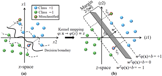
In situation where the classes overlap separating the classes by boundary linear decision-making is always flawed. In order to overcome this issue, we can start using initial data from the Rn dimension using a nonlinear transformation , moved to the Rm dimension, in the dimensions that classes have fewer interference with each other. In this case, finding the optimal decision boundary for solving the optimization problem is as follows:
In this optimization problem αi.α is Lagrange multipliers and c are constant values. In formula (2) Instead of using it's better to use a core function which is determined as follows:
After defining the right k (xi, xj), in formula (2) instead of (xi) (xj), the function k (xi, xj) remodeled and optimization problem can be solved. One of the useful core functions is sigmoid kernel function which is explained as follows (Huang et al., 2005; Vapnik, 1995, 1998):
C and γ are two important parameters of SVM, which should be chosen very carefully. Parameter C indicates the penalty. If C is assigned a large value, the accuracy rate of the classification will be higher and lower correspondingly in the training phase and the test phase which is called over fitting. On the other hand, if the value of C is small, the classification accuracy will be inadequate. A similar scenario applies to γ, but it has a deeper effect than C in the results because it affects the feature space of the result.
3.2 SVM and PSO
PSO was introduced in 1995 by Kennedy and Eberhart according to the social simulation model known as a stochastic optimization algorithm (Jamous, 2015). Research and applications on particle swarm optimization PSO have increased quickly due to its formation which has resulted in many improved PSO algorithms for various kinds of optimization problems. In PSO, the hyper-parameter is optimized by two features; the algorithm and its function (Pandith, 2016; Wang, 2017). In one research, PSO algorithms simulate the behavior of a bird flock by simulating the accuracy of intervals between birds and members which could be dependent on the physical appearance and its performance. Each bird in the area of searching is called a particle which is considered a single resolution. Each particle has its own function value that should be evaluated and optimized and lead by the velocity of the best particle (Jamous, 2015; Chen et al., 2008). This is applied in PSO algorithms to enhance the original PSO or address the optimization issues. Lots of work and study on the effectiveness of PSO compared to other machine learning and swarm intelligence algorithm for engineering and computer science problems have been done by researchers to evaluate its performances (Bashath and Ismail, 2018). As can be seen in in Figure 2 the optimized algorithm has outperformed the other algorithms in both sets of experiments.
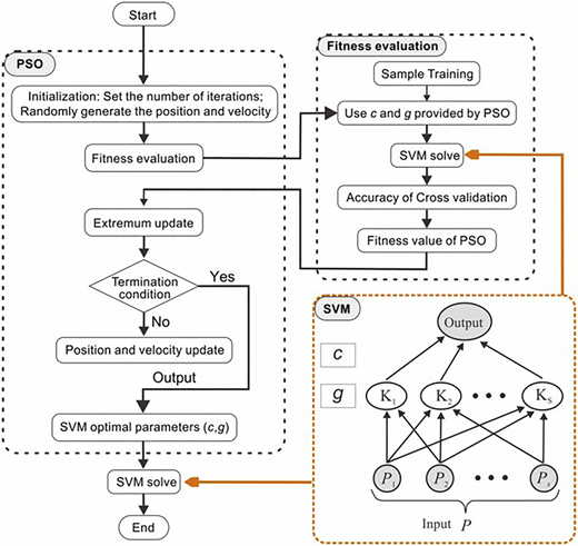
Figure 3 shows that the preparation of PSO with population size, inaction weight and generations without improvements. After evaluating of each particle, the fitness functions and the local best and global best parameters will be compared. Once finished, the velocity and position of each particle will be updated until the value of the fitness task converges. After converging, the global best particle in the swarm is fed to the SVM classifier for training. Finally, the SVM classifier will be trained (Basari et al., 2013).
4. Methodology
The purpose of this study is to use an appropriate structure to predict the trading signals of the stock market with high precision. For this purpose, regarding the background presented in the previous chapter, in this study, one model is used to analyze the technical adaptation. The model is described in two separate sections.
4.1 Input data
The input dataset used in this study, is based on the two approaches introduced for the first time by Jasemi et al. (2011a, b). In these two approaches, the daily stock prices including low, high, open and close prices turn into 15 and 24 indicators based on what is shown in Tables 1 and 2, respectively for the first and second approaches. It is to be noted that in the tables , , and respectively denotes open, high, low and close prices on the ith day while 7th day is today (last day), 6th day is yesterday and so on. The output is stock performance that is given in the form of buy, sell or no-action signal.
Table 3 describes the 4 datasets that are used on a daily basis for model training and testing. Each dataset is divided into two groups of training and testing sets and each set contains daily stock prices. For example, in dataset 1, data of year 2013 is used for training and data of year 2014 is used for testing. In dataset 2, time-distance between training and test data are increased and data of year 2015 are used for testing. In other datasets the number of training data is also increased; for example, in dataset 9, data of year 2013 and 2014 are used together as a single training data.
Details of training and checking of the applied data sets. (2013 to 2021)
| No | Training period | Test period | No | Training period | Test period | No. | Training period | Test period | No. | Training period | Test period |
|---|---|---|---|---|---|---|---|---|---|---|---|
| 1 | 2013 | 2014 | 13 | 2013–2014 | 2019 | 25 | 2013–2016 | 2020 | 37 | 2014–2015 | 2019 |
| 2 | 2013 | 2015 | 14 | 2013–2014 | 2020 | 26 | 2013–2016 | 2021 | 38 | 2014–2015 | 2020 |
| 3 | 2013 | 2016 | 15 | 2013–2014 | 2021 | 27 | 2014 | 2015 | 39 | 2014–2015 | 2021 |
| 4 | 2013 | 2017 | 16 | 2013–2015 | 2016 | 28 | 2014 | 2016 | 40 | 2014–2016 | 2017 |
| 5 | 2013 | 2018 | 17 | 2013–2015 | 2017 | 29 | 2014 | 2017 | 41 | 2014–2016 | 2018 |
| 6 | 2013 | 2019 | 18 | 2013–2015 | 2018 | 30 | 2014 | 2018 | 42 | 2014–2016 | 2019 |
| 7 | 2013 | 2020 | 19 | 2013–2015 | 2019 | 31 | 2014 | 2019 | 43 | 2014–2016 | 2020 |
| 8 | 2013 | 2021 | 20 | 2013–2015 | 2020 | 32 | 2014 | 2020 | 44 | 2014–2016 | 2021 |
| 9 | 2013–2014 | 2015 | 21 | 2013–2015 | 2021 | 33 | 2014 | 2021 | 45 | 2014–2017 | 2018 |
| 10 | 2013–2014 | 2016 | 22 | 2013–2016 | 2017 | 34 | 2014–2015 | 2003 | 46 | 2014–2017 | 2019 |
| 11 | 2013–2014 | 2017 | 23 | 2013–2016 | 2018 | 35 | 2014–2015 | 2004 | 47 | 2014–2017 | 2020 |
| 12 | 2013–2014 | 2018 | 24 | 2013–2016 | 2019 | 36 | 2014–2015 | 2005 | 48 | 2014–2017 | 2021 |
4.2 The introduction of the model
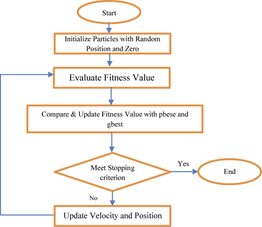
The optimization method that we have used in this article is the PSO method, PSO is a relatively new heuristic search method derived from the behavior of social groups such as flock of birds and fish swarms. PSO uses a combination of deterministic and probabilistic rules to switch from one set of points to another set of points in single iteration that can be improved. PSO is popular in academia and industry, primarily due to its intuition, ease of implementation and ability to effectively solve the highly nonlinear mixed integer optimization problems that are typical engineering systems. Although the “survival of the fittest” principle is not used in PSO, it is usually considered as an evolutionary algorithm. Optimization is achieved by providing each individual in the search space with a memory of previous success, information about the success of social groups, and the possibility of incorporating this knowledge into the individual's movements.
Hence, each individual (called particle) is characterized by its position , its velocity , its personal best position and its neighborhood best position . The elements of the velocity vector for particle i are updated as:
Where w is the inertia weight, is the best variable vector encountered so far by particle i, and. is the swarm best vector, i.e. the best variable vector found by any particle in the swarm, so far and are constants, and q and r are random numbers in the range (0, 1). Once the velocities have been updated, the variable vector of particle i is modified according to:
The cycle of evaluation followed by updates of velocities and positions (and possible update of and) is then repeated until a satisfactory solution is found. In Figure 3 PSO algorithm is shown (Hegazy et al., 2013).
4.2.1 SVM-PSO
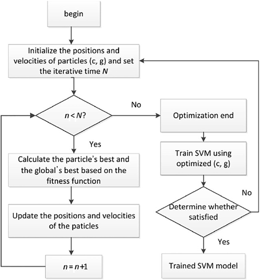
The SVM method is based on the VC dimension theory and the structural risk minimization principle (Cortes and Vapnik, 1995). It classifies two types by transforming the data to a higher dimensional feature space to find the optimal hyperplane in the space which maximizes the margin between the two types.
The parameters in the SVM have a significant influence on the classification result. However, the parameter selection lacks theoretical guidance. The PSO is a computational intelligence method that is motivated by organisms' behaviors, such as the flocking of birds. It has a well-balanced mechanism to enhance global and local exploration abilities. So the PSO was used to select the penalty parameter c and the kernel parameter g in the SVM with a Gaussian kernel. In the PSO, (c, g) become the particles (Xue et al., 2020).
The PSO-SVM is briefly introduced as follows:
Initialize the particles (c, g) and the iterative time N.
Calculate the objective function value of the particle using the SVM training algorithm.
Calculate the optimal historical values of the individual and the population.
Update the particle velocity and position according to the speed and position update equations.
If the iterative time is satisfied, output the optimal parameters; otherwise, go back to step 3.
If the SVM accuracy does not meet the requirement, go back to step 1.
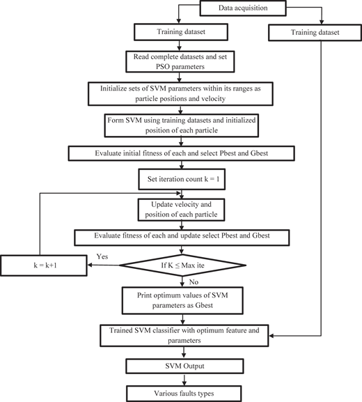
The flowchart of the PSO-SVM is shown in Figure 4.
The detailed experimental procedure for feature extraction and SVM parameter selection using PSO algorithm can be represented by the following procedure.
Read complete data and set , and parameters.
Initialize positions X and velocities V of each particle of population.
Initialize sets of SVM parameters within its ranges as particle position and velocity.
Form SVM using training dataset and initialized positions of each particle.
Evaluate fitness of each particle = (), , and find the best particle index .
Select = , and = .
Set iteration count .
= max − ( max − min) × ite/max ite.
Update velocity and position of each particle using (14) and (15).
Evaluate updated fitness of each particle = (), , and find the best particle index .
Update of each particle If < then = ;
Else = .
Update of population If < then < and set ; else < .
If max ite then and go to step (6); else go to step (14).
Optimum solution obtained: print the results of optimum generation as .
Retrain SVM with optimum features and parameters; then identify unknown samples on testing dataset.
Data may vary based on the datasets available from the source. This covers not only the opening/closing prices, but also the highest/lowest prices of the day. The experiment procedure can be visualized in Figure 5.
4.2.2 Algorithm SVM-PSO
In this article, according to the modeling conditions and in order to achieve optimal results the following pseudo-code is used. Based on its implementation in python programming language, we have reached results that will be briefly explained in the next section. According to the pseudo-code, in the particles matrix, the first row is for parameter C, the second row is for gamma parameter of SVM algorithm and the rest of the rows are the presence and absence of the corresponding feature in raw approach and signal approach. In other word, matrix in raw approach has 17 rows and in signal approach has 26 rows. For the row related to the features, if the corresponding entry in the matrix is greater than 0.5, then the feature will be present in the presence algorithm, otherwise it will be deleted. It should be noted that according to experimental observations the values of and, which are equivalent to the initial minimum values and the maximum value for the C parameter of the SVM algorithm respectively, play an important role in obtaining the optimal answer. In the experimental related to one-day data from the parameters = 2.5, = 1.5, = 0.4, = 1.4, = 0, = 100 and from 18 particles and for 6-day data from the same input parameters with the difference that is used. The input data used are from the Yahoo finance site between 2013 and 2021. In case of further studies, the data of this period along with the code of this model will be provided to researchers for free.Table 9
4.3 Calculate the total number of signals and hit rate
Performance measures can be categorized into two groups of statistical and nonstatistical ones. Nonstatistical measures cover the economic aspects. In the area of this paper, the statistical ones are more common while the most popular one is hit rate (Atsalakis and Valavanis, 2009). Hit rate is defined as (number of success)/(total signals). If the hit rate is higher than 51%, it is considered as a useful model (Lee, 2009).
At this stage, with model outputs, sell and buy signals and total number of signals are figured out and the number of correct signals during a 6-day period is calculated. Since the base or standard study is Jasemi et al. (2011a, b), every details are set according to that study and reading that paper is recommended for better understanding.
5. Results and discussion
5.1 Experimental results of SVM-PSO
The implementation of the algorithm for the raw and signal approaches, optimization parameters of Radial basis function (RBF) and the results for 48 datasets, are shown in Table 4. This table shows the output of the algorithm, including the optimal parameters (C, σ), feature numbers and the achieved hit rate (accuracy). Results of accuracy are the hit rates associated with the first and second approaches which can be seen in Tables 4 and 5, respectively.
Results of accuracy of the implementation SVM-PSO model Raw Approach
| No. | C | σ | Feature numbers | Accuracy | No. | C | σ | Feature numbers | Accuracy |
|---|---|---|---|---|---|---|---|---|---|
| 1 | 13/4 | 0/3 | 80/2 | 9 | 25 | 58/7 | 0/3 | 80/8 | 8 |
| 2 | 7/8 | 0/8 | 73/4 | 9 | 26 | 34/5 | 0/8 | 73/4 | 7 |
| 3 | 17/9 | 0/3 | 79/8 | 6 | 27 | 97/6 | 70/3 | 79/8 | 7 |
| 4 | 64/5 | 0/3 | 79/3 | 6 | 28 | 8452037/6 | 0/6 | 80/9 | 8 |
| 5 | 39/1 | 0/5 | 74/1 | 6 | 29 | 48/9 | 36/6 | 74/9 | 7 |
| 6 | 27/8 | 0/2 | 77/8 | 7 | 30 | 5/4 | 0/1 | 77/8 | 6 |
| 7 | 42/7 | 0/7 | 75/9 | 6 | 31 | 11/9 | 0/5 | 75/9 | 8 |
| 8 | 13/1 | 0/2 | 80/8 | 6 | 32 | 64/2 | 0/3 | 80/8 | 8 |
| 9 | 84/9 | 0/8 | 73/4 | 10 | 33 | 6241061/3 | 0/4 | 80/2 | 6 |
| 10 | 48/7 | 0/3 | 79/8 | 11 | 34 | 75/1 | 0/1 | 79/3 | 6 |
| 11 | 3/8 | 0/0 | 79/3 | 7 | 35 | 11/4 | 0/5 | 74/1 | 10 |
| 12 | 29/7 | 0/4 | 74/1 | 7 | 36 | 20/7 | 0/0 | 77/8 | 7 |
| 13 | 23/1 | 0/6 | 77/8 | 6 | 37 | 6/9 | 0/3 | 75/9 | 7 |
| 14 | 90744/1 | 0/7 | 77/5 | 7 | 38 | 18/1 | 0/7 | 80/8 | 9 |
| 15 | 168243/8 | 1/1 | 81/7 | 8 | 39 | 28/8 | 0/5 | 79/3 | 9 |
| 16 | 57/0 | 151/1 | 80/2 | 5 | 40 | 34/7 | 0/2 | 74/1 | 5 |
| 17 | 59/2 | 67/4 | 80/1 | 10 | 41 | 36/2 | 0/4 | 77/8 | 8 |
| 18 | 25/1 | 0/0 | 74/1 | 7 | 42 | 15/4 | 0/6 | 75/9 | 6 |
| 19 | 61/7 | 0/1 | 77/8 | 4 | 43 | 7/0 | 220/3 | 81/3 | 7 |
| 20 | 182569/7 | 0/9 | 78/3 | 6 | 44 | 4/3 | 353/9 | 75/3 | 9 |
| 21 | 20/6 | 0/8 | 80/8 | 8 | 45 | 52/1 | 0/2 | 77/8 | 7 |
| 22 | 6/5 | 0/4 | 79/3 | 6 | 46 | 15/1 | 214/6 | 77/1 | 6 |
| 23 | 96/4 | 81/1 | 74/9 | 9 | 47 | 6/6 | 0/2 | 80/8 | 6 |
| 24 | 19/5 | 0/7 | 77/8 | 4 | 48 | 58/7 | 0/3 | 80/8 | 8 |
Results of accuracy of the implementation SVM-PSO model signal approach
| No | C | σ | Feature numbers | Accuracy | No | C | σ | Feature numbers | Accuracy |
|---|---|---|---|---|---|---|---|---|---|
| 1 | 18/5 | 0/4 | 80/2 | 9 | 25 | 71/6 | 0/3 | 80/8 | 11 |
| 2 | 78/2 | 0/6 | 73/4 | 11 | 26 | 25/0 | 0/2 | 73/4 | 10 |
| 3 | 44/8 | 24/9 | 80/2 | 15 | 27 | 17/3 | 0/3 | 79/8 | 6 |
| 4 | 17/7 | 87/5 | 80/5 | 14 | 28 | 52/8 | 0/0 | 79/3 | 12 |
| 5 | 1774124/0 | 0/3 | 75/7 | 10 | 29 | 33/2 | 0/1 | 74/1 | 9 |
| 6 | 391302/4 | 0/4 | 78/6 | 13 | 30 | 43/7 | 0/6 | 77/8 | 12 |
| 7 | 62/2 | 0/2 | 75/9 | 11 | 31 | 3/5 | 0/3 | 75/9 | 11 |
| 8 | 144728/3 | 0/9 | 81/3 | 10 | 32 | 146/2 | 14/9 | 82/2 | 14 |
| 9 | 123/5 | 234/4 | 75/4 | 10 | 33 | 14/1 | 0/4 | 79/8 | 16 |
| 10 | 42/9 | 0/1 | 79/8 | 8 | 34 | 87/8 | 70/7 | 80/5 | 12 |
| 11 | 5/1 | 220/3 | 80/5 | 13 | 35 | 41/7 | 0/1 | 74/1 | 14 |
| 12 | 18/3 | 0/2 | 74/1 | 5 | 36 | 25/1 | 0/0 | 77/8 | 11 |
| 13 | 1312753/4 | 0/3 | 79/0 | 16 | 37 | 86/9 | 0/2 | 75/9 | 9 |
| 14 | 27/1 | 0/3 | 75/9 | 10 | 38 | 1024654/2 | 0/9 | 81/7 | 7 |
| 15 | 25/4 | 0/2 | 80/8 | 9 | 39 | 76/1 | 278/9 | 80/1 | 9 |
| 16 | 10/8 | 0/1 | 79/8 | 8 | 40 | 58/3 | 0/3 | 74/1 | 10 |
| 17 | 67/0 | 122/5 | 80/5 | 11 | 41 | 73/8 | 0/2 | 77/8 | 15 |
| 18 | 6/2 | 87/9 | 75/3 | 14 | 42 | 6/6 | 0/0 | 75/9 | 12 |
| 19 | 3/3 | 0/1 | 77/8 | 12 | 43 | 98/8 | 18/5 | 80/8 | 12 |
| 20 | 38/7 | 0/4 | 75/9 | 7 | 44 | 7/6 | 0/3 | 74/1 | 12 |
| 21 | 54/1 | 0/6 | 80/8 | 14 | 45 | 4/5 | 0/2 | 77/8 | 10 |
| 22 | 11/5 | 201/3 | 80/5 | 12 | 46 | 251/4 | 104/1 | 77/9 | 8 |
| 23 | 12/5 | 0/5 | 74/1 | 12 | 47 | 25/5 | 0/7 | 80/8 | 12 |
| 24 | 60/2 | 0/2 | 77/8 | 13 | 48 | 71/6 | 0/3 | 80/8 | 11 |
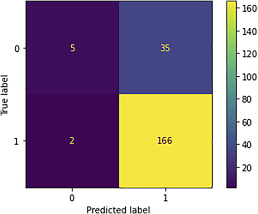
As an example, the diagonal of the matrix output shows the number of right signals and other elements of the matrix show the number of target signals that were predicted by mistake. There are two classes of ascending, neutral and descending signals predicted by the model in this matrix. Total of rows 1 and 2 elements indicates the number of ascending, neutral and descending signals respectively. In this matrix, the total number of forecasts and the number of correct forecasts are displayed in each row. Note that the matrix is created for each dataset.
Figure 6 shows the prediction accuracy by PSO with the two approaches. According to it, the labeled data are sell, buy and neutral signals. To obtain them, the financial return of the close price of the signal day is calculated as follows:
Where CP is the close price, and t0 is the time interval between the signal day and the next day(s). In this study, six different time intervals ranging from one to six days are considered, and the corresponding financial returns are calculated. Following that, a signal is considered to be sell or buy signal if it has positive or negative financial return, respectively. However, to increase reliability, a lower bound of mp for the positive returns and an upper bound of for negative returns is applied. Where mp is means of positive daily return and mn is means of negative daily return of the stock during the test year.
Based on the description above, the achieved values are obtained in this order. It is obvious that the accuracy of SVM by signal approach is higher than raw approach for most of the datasets. Additionally, the average accuracy of 48 datasets in the first and the second approaches are 76 and 79%, respectively.
Figures 7 and 8 show the total number of signals in both approaches, Raw approach and Signal approach respectively to present better depiction of the results.
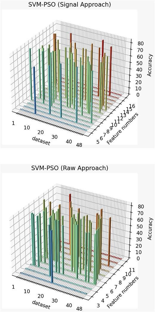
(Raw Approach) as the following image, highest accuracy is for the 43 datasets which use 7 feature and has an accuracy of 82.58%. In addition, it can be seen that in most datasets (14 times) six features are used and it shows the best performance. The accuracy of 48 datasets is 77.23% on average.
(Signal Approach) As can be seen in image, the highest accuracy belongs to 32 datasets, which use 7 features and has an accuracy of 83.62%. Moreover, it is obvious that in most datasets (9 times) up to 11 features have been used and it shows the best performance. The accuracy in 48 datasets is 77.40% on average.
Figure 7 shows the total number of signals in both approaches the raw approach, and the signal approach respectively, to present better depiction of the results.
Table 6 displays the hit rate for periods of 1 and 6 days as well as the total number of buying and selling signals. Table 7 displays the complete list of results while columns 1 to 6 represent the percentages of correct signals on one, two, three, four, five and six-day periods, respectively. Column 7 shows the total number of right signals and column 8 relates to the total number of signals emitted by the model.
Hit Rate for 1 and 6 day periods by SVM-PSO model in both approaches
| Raw approach | Signal approach | ||||||||||||||
|---|---|---|---|---|---|---|---|---|---|---|---|---|---|---|---|
| No. | 1d (%) | 6d (%) | Sig. no. | No. | 1d (%) | 6d (%) | Sig. no. | No. | 1d (%) | 6d (%) | Sig. no. | No. | 1 d (%) | 6d (%) | Sig. no. |
| 1 | 0.20 | 0.91 | 86 | 25 | 0.25 | 0.75 | 32 | 1 | 0.23 | 0.87 | 30 | 25 | 0.00 | 0.33 | 3 |
| 2 | 0.25 | 0.94 | 72 | 26 | 0.50 | 0.80 | 10 | 2 | 0.09 | 0.77 | 35 | 26 | - | - | 0 |
| 3 | 0.12 | 0.54 | 84 | 27 | 0.08 | 0.67 | 12 | 3 | 0.31 | 0.71 | 35 | 27 | 0.36 | 0.86 | 145 |
| 4 | 0.07 | 0.75 | 59 | 28 | 0.00 | 0.44 | 9 | 4 | 0.16 | 0.65 | 51 | 28 | 0.22 | 0.71 | 99 |
| 5 | 0.30 | 0.93 | 30 | 29 | 0.00 | 0.56 | 16 | 5 | 0.22 | 0.74 | 50 | 29 | 0.17 | 0.59 | 46 |
| 6 | 0.11 | 0.91 | 88 | 30 | 0.26 | 0.47 | 34 | 6 | 0.26 | 0.85 | 34 | 30 | 0.25 | 0.78 | 120 |
| 7 | 0.10 | 0.77 | 70 | 31 | 0.33 | 0.83 | 30 | 7 | 0.27 | 0.69 | 26 | 31 | 0.34 | 0.93 | 143 |
| 8 | 0.46 | 0.92 | 13 | 32 | 0.23 | 0.74 | 53 | 8 | 0.50 | 1.00 | 16 | 32 | 0.25 | 0.91 | 53 |
| 9 | 0.25 | 0.85 | 20 | 33 | 0.17 | 0.50 | 64 | 9 | 0.18 | 0.65 | 17 | 33 | 1.00 | 1.00 | 1 |
| 10 | 0.16 | 0.57 | 51 | 34 | 0.29 | 0.71 | 21 | 10 | 0.29 | 0.67 | 72 | 34 | 0.25 | 0.74 | 65 |
| 11 | 0.14 | 0.57 | 28 | 35 | 0.07 | 0.36 | 14 | 11 | 0.20 | 0.71 | 45 | 35 | 0.13 | 0.58 | 53 |
| 12 | 0.22 | 0.54 | 37 | 36 | 0.24 | 0.66 | 29 | 12 | 0.22 | 0.80 | 41 | 36 | 0.23 | 0.77 | 110 |
| 13 | 0.23 | 0.72 | 61 | 37 | 0.13 | 0.58 | 24 | 13 | 0.36 | 0.87 | 39 | 37 | 0.36 | 0.96 | 118 |
| 14 | 0.21 | 0.76 | 63 | 38 | 0.15 | 0.65 | 20 | 14 | 0.16 | 0.79 | 19 | 38 | 0.28 | 0.85 | 127 |
| 15 | 0.50 | 0.93 | 14 | 39 | 0.29 | 1.00 | 14 | 15 | 0.00 | 1.00 | 1 | 39 | 0.50 | 1.00 | 4 |
| 16 | 0.19 | 0.43 | 21 | 40 | 0.09 | 0.55 | 11 | 16 | 0.27 | 0.64 | 75 | 40 | 0.14 | 0.59 | 56 |
| 17 | 0.00 | 0.31 | 13 | 41 | 0.30 | 0.57 | 23 | 17 | 0.24 | 0.71 | 59 | 41 | 0.24 | 0.77 | 112 |
| 18 | 0.17 | 0.75 | 12 | 42 | 0.18 | 0.68 | 38 | 18 | 0.24 | 0.78 | 55 | 42 | 0.43 | 0.98 | 56 |
| 19 | 0.23 | 0.60 | 40 | 43 | 0.17 | 0.72 | 53 | 19 | 0.31 | 0.84 | 55 | 43 | 0.27 | 0.83 | 111 |
| 20 | 0.14 | 0.72 | 57 | 44 | 0.11 | 0.78 | 9 | 20 | 0.35 | 0.85 | 26 | 44 | 0.00 | 1.00 | 1 |
| 21 | 0.56 | 0.78 | 9 | 45 | 0.33 | 0.33 | 3 | 21 | 0.25 | 1.00 | 4 | 45 | 0.26 | 0.79 | 114 |
| 22 | 0.10 | 0.40 | 10 | 46 | 0.17 | 0.63 | 52 | 22 | 0.17 | 0.50 | 12 | 46 | 0.37 | 0.93 | 30 |
| 23 | 0.50 | 0.67 | 6 | 47 | 0.16 | 0.68 | 74 | 23 | 0.23 | 0.77 | 22 | 47 | 0.32 | 0.86 | 107 |
| 24 | 0.29 | 0.75 | 24 | 48 | 0.09 | 0.73 | 11 | 24 | 0.33 | 1.00 | 6 | 48 | 0.00 | 1.00 | 2 |
The complete list of the results
| Raw approach | Signal approach | ||||||||||||||||
|---|---|---|---|---|---|---|---|---|---|---|---|---|---|---|---|---|---|
| No. | 1 | 2 | 3 | 4 | 5 | 6 | 7 | 8 | No. | 1 | 2 | 3 | 4 | 5 | 6 | 7 | 8 |
| 1 | 17 | 13 | 17 | 11 | 8 | 12 | 78 | 86 | 1 | 7 | 7 | 7 | 2 | 2 | 1 | 26 | 30 |
| 2 | 18 | 8 | 15 | 12 | 9 | 6 | 68 | 72 | 2 | 3 | 7 | 6 | 5 | 4 | 2 | 27 | 35 |
| 3 | 10 | 7 | 8 | 8 | 5 | 7 | 45 | 84 | 3 | 11 | 5 | 3 | 2 | 1 | 3 | 25 | 35 |
| 4 | 4 | 7 | 6 | 13 | 7 | 7 | 44 | 59 | 4 | 8 | 7 | 6 | 5 | 4 | 3 | 33 | 51 |
| 5 | 9 | 5 | 3 | 5 | 3 | 3 | 28 | 30 | 5 | 11 | 8 | 7 | 4 | 3 | 4 | 37 | 50 |
| 6 | 10 | 15 | 10 | 15 | 13 | 17 | 80 | 88 | 6 | 9 | 9 | 3 | 4 | 2 | 2 | 29 | 34 |
| 7 | 7 | 10 | 7 | 10 | 10 | 10 | 54 | 70 | 7 | 7 | 4 | 2 | 3 | 1 | 1 | 18 | 26 |
| 8 | 6 | 3 | 1 | 1 | 1 | 0 | 12 | 13 | 8 | 8 | 2 | 3 | 2 | 1 | 0 | 16 | 16 |
| 9 | 5 | 5 | 5 | 1 | 0 | 1 | 17 | 20 | 9 | 3 | 4 | 2 | 2 | 0 | 0 | 11 | 17 |
| 10 | 8 | 6 | 5 | 3 | 6 | 1 | 29 | 51 | 10 | 21 | 11 | 8 | 4 | 1 | 3 | 48 | 72 |
| 11 | 4 | 3 | 2 | 4 | 2 | 1 | 16 | 28 | 11 | 9 | 11 | 6 | 3 | 3 | 0 | 32 | 45 |
| 12 | 8 | 5 | 2 | 3 | 0 | 2 | 20 | 37 | 12 | 9 | 8 | 4 | 5 | 2 | 5 | 33 | 41 |
| 13 | 14 | 7 | 11 | 8 | 2 | 2 | 44 | 61 | 13 | 14 | 7 | 5 | 3 | 4 | 1 | 34 | 39 |
| 14 | 13 | 10 | 10 | 7 | 7 | 1 | 48 | 63 | 14 | 3 | 3 | 4 | 0 | 3 | 2 | 15 | 19 |
| 15 | 7 | 2 | 1 | 1 | 2 | 0 | 13 | 14 | 15 | 0 | 1 | 0 | 0 | 0 | 0 | 1 | 1 |
| 16 | 4 | 1 | 1 | 2 | 1 | 0 | 9 | 21 | 16 | 20 | 10 | 8 | 4 | 3 | 3 | 48 | 75 |
| 17 | 0 | 1 | 2 | 1 | 0 | 0 | 4 | 13 | 17 | 14 | 12 | 5 | 7 | 3 | 1 | 42 | 59 |
| 18 | 2 | 2 | 1 | 1 | 1 | 2 | 9 | 12 | 18 | 13 | 9 | 7 | 4 | 5 | 5 | 43 | 55 |
| 19 | 9 | 2 | 5 | 5 | 1 | 2 | 24 | 40 | 19 | 17 | 9 | 3 | 7 | 6 | 4 | 46 | 55 |
| 20 | 8 | 10 | 10 | 7 | 5 | 1 | 41 | 57 | 20 | 9 | 5 | 3 | 1 | 3 | 1 | 22 | 26 |
| 21 | 5 | 1 | 1 | 0 | 0 | 0 | 7 | 9 | 21 | 1 | 1 | 1 | 1 | 0 | 0 | 4 | 4 |
| 22 | 1 | 1 | 0 | 1 | 1 | 0 | 4 | 10 | 22 | 2 | 2 | 0 | 1 | 0 | 1 | 6 | 12 |
| 23 | 3 | 0 | 1 | 0 | 0 | 0 | 4 | 6 | 23 | 5 | 3 | 3 | 2 | 2 | 2 | 17 | 22 |
| 24 | 7 | 2 | 3 | 3 | 2 | 1 | 18 | 24 | 24 | 2 | 1 | 0 | 1 | 1 | 1 | 6 | 6 |
| 25 | 8 | 2 | 7 | 3 | 2 | 2 | 24 | 32 | 25 | 0 | 0 | 0 | 0 | 1 | 0 | 1 | 3 |
| 26 | 5 | 2 | 1 | 0 | 0 | 0 | 8 | 10 | 26 | 0 | 0 | 0 | 0 | 0 | 0 | 0 | 0 |
| 27 | 1 | 2 | 5 | 0 | 0 | 0 | 8 | 12 | 27 | 52 | 31 | 17 | 15 | 6 | 4 | 125 | 145 |
| 28 | 0 | 2 | 0 | 1 | 1 | 0 | 4 | 9 | 28 | 22 | 14 | 15 | 7 | 6 | 6 | 70 | 99 |
| 29 | 0 | 3 | 0 | 3 | 2 | 1 | 9 | 16 | 29 | 8 | 7 | 4 | 6 | 2 | 0 | 27 | 46 |
| 30 | 9 | 1 | 0 | 2 | 2 | 2 | 16 | 34 | 30 | 30 | 21 | 13 | 13 | 10 | 7 | 94 | 120 |
| 31 | 10 | 5 | 5 | 3 | 1 | 1 | 25 | 30 | 31 | 49 | 31 | 20 | 13 | 12 | 8 | 133 | 143 |
| 32 | 12 | 5 | 7 | 7 | 5 | 3 | 39 | 53 | 32 | 13 | 6 | 5 | 10 | 10 | 4 | 48 | 53 |
| 33 | 11 | 7 | 6 | 5 | 2 | 1 | 32 | 165 | 33 | 1 | 0 | 0 | 0 | 0 | 0 | 1 | 1 |
| 34 | 6 | 3 | 1 | 3 | 2 | 0 | 15 | 21 | 34 | 16 | 8 | 8 | 7 | 5 | 4 | 48 | 65 |
| 35 | 1 | 1 | 1 | 0 | 1 | 1 | 5 | 14 | 35 | 7 | 7 | 3 | 3 | 8 | 3 | 31 | 53 |
| 36 | 7 | 4 | 2 | 3 | 1 | 2 | 19 | 29 | 36 | 25 | 16 | 18 | 13 | 8 | 5 | 85 | 110 |
| 37 | 3 | 0 | 4 | 4 | 2 | 1 | 14 | 24 | 37 | 42 | 24 | 15 | 15 | 11 | 6 | 113 | 118 |
| 38 | 3 | 0 | 4 | 3 | 2 | 1 | 13 | 20 | 38 | 36 | 22 | 13 | 20 | 13 | 4 | 108 | 127 |
| 39 | 4 | 2 | 5 | 2 | 1 | 0 | 14 | 14 | 39 | 2 | 0 | 2 | 0 | 0 | 0 | 4 | 4 |
| 40 | 1 | 1 | 0 | 1 | 2 | 1 | 6 | 11 | 40 | 8 | 5 | 5 | 5 | 8 | 2 | 33 | 56 |
| 41 | 7 | 0 | 1 | 2 | 2 | 1 | 13 | 23 | 41 | 27 | 10 | 18 | 15 | 10 | 6 | 86 | 112 |
| 42 | 7 | 4 | 6 | 4 | 3 | 2 | 26 | 38 | 42 | 24 | 9 | 5 | 9 | 4 | 4 | 55 | 56 |
| 43 | 9 | 5 | 9 | 9 | 1 | 5 | 38 | 53 | 43 | 30 | 17 | 11 | 18 | 12 | 4 | 92 | 111 |
| 44 | 1 | 3 | 2 | 1 | 0 | 0 | 7 | 9 | 44 | 0 | 0 | 1 | 0 | 0 | 0 | 1 | 1 |
| 45 | 1 | 0 | 0 | 0 | 0 | 0 | 1 | 3 | 45 | 30 | 17 | 18 | 13 | 9 | 3 | 90 | 114 |
| 46 | 9 | 8 | 5 | 6 | 2 | 3 | 33 | 52 | 46 | 11 | 5 | 3 | 4 | 3 | 2 | 28 | 30 |
| 47 | 12 | 10 | 9 | 11 | 3 | 5 | 50 | 74 | 47 | 34 | 19 | 12 | 19 | 5 | 3 | 92 | 107 |
| 48 | 1 | 3 | 1 | 1 | 1 | 1 | 8 | 11 | 48 | 0 | 0 | 1 | 1 | 0 | 0 | 2 | 2 |
6. Validation
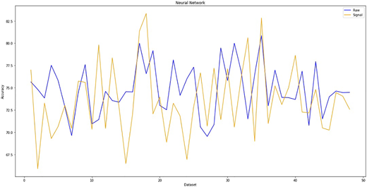
In order to examine the reliability and accuracy of the model, we compare the performance of the proposed PSO algorithm with the results of Jasemi's model which was solved by neural network with similar input data. According to the neural networks model of Milad et al. and comparing their one and two attitudes, we reach the following diagram in Figure 8, which shows the accuracy of the neural networks in the two approaches (raw approach & signal approach).
Table 8 illustrate how the SVM-PSO approach is superior to the neural networks (the base study). In the SVM-PSO model, the hit rate raw approach is 79% and it is to be noted that the SVM-PSO got the fantastic average hit rate signal approach of 76% when the second approach is applied. Eventually, the total hit rate is 77.5%, which is better than the hit rate of a neural network.
Comparing the models with two approaches
| Models | Total hit ratio (%) | Hit ratio raw approach (%) | Hit ratio signal approach (%) | Hit ratio 1-day/raw approach (%) | Hit ratio 1-day/signal approach (%) |
|---|---|---|---|---|---|
| Neural Network | 74.2 | 74.8 | 73.6 | 45 | 43.4 |
| SVM-PSO | 77.5 | 78.5 | 74.2 | 47.6 | 43.8 |
This research proposed a new model for stock market timing in the way that SVM is a classifier and PSO is used for the optimization of the SVM parameters. PSO also chooses the optimum features for better forecasting. To make the comparison fair, all the details are set according to the case study. So a 6-day long time period is considered for evaluation of the proposed new model. Table 8 shows an overall comparison between the two models (the base study and the newly proposed model in this study). The results show that while SVM-PSO is superior to the basic study, the new model is reliable and stable over 6 days.
7. Conclusion
This research proposed a new model for stock market timing in the way that SVM is a classifier and PSO is used for the optimization of the SVM parameters. PSO also chooses the optimum features for better forecasting. To make the comparison fair, all the details are set according to the case study. So a 6-day long time period is considered for evaluation of the proposed new model. The results show that while SVM-PSO is superior to the basic study, it is reliable and stable over 6 days. In detail, their differences become significant when the hit ratio is investigated during a day. In both approaches, the SVM-PSO by 77.5% accuracy performance is the leader in general, but in the signal approach, the hit ratio in SVM-PSO has a slight difference by day, approximately 0.5%, which cannot be considered as a significant improvement in the prediction of the model. Hence, from this perspective, the signal approach needs to be changed by choosing the type of nodes in the return signal or the number of them. However, this comparison for the raw approach depicts that the SVM-PSO model works successfully in both periods of time whether the whole 6-day period or one day, 78.5% and 47.6% respectively.
