


The reduced problem of the Navier–Stokes and the continuity equations, in two-dimensional Cartesian coordinates with Eulerian description, for incompressible non-Newtonian fluids, is considered. The Ladyzhenskaya model, with a non-linear velocity dependent stress tensor is adopted, and leads to the governing equation of interest. The reduction is based on a self-similar transformation as demonstrated in existing literature, for two spatial variables and one time variable, resulting in an ODE defined on a semi-infinite domain. In our search for classical solutions, existence and uniqueness will be determined depending on the signs of two parameters with physical interpretation in the equation. Illustrations are included to highlight some of the main results.
1. Introduction
The study of non-Newtonian fluids, both mathematically and physically, has gained much importance during the last few decades due to their many applications in industry and in describing physical phenomena. The basic physical theory, and its mathematical formulation can be found in [1,8,18]. Many researchers studied non-Newtonian fluids from a numerical or computational point of view, in some instances accompanied with certain techniques or transformations to elucidate investigating the problem [6,9]. Other studies involved existence and uniqueness of solutions to problems involving non-Newtonian fluids [10,11,20,21]. Many times, it is found that solutions for Newtonian and non-Newtonian flows are not unique [7,13,15,17]. In some instances or special cases, exact solutions were established, see for example [12]. Our interest in this paper is in a Ladyzhenskaya type non-Newtonian fluid [16], where self-similar transformations of the Navier–Stokes equations, for non-Newtonian incompressible fluids, lead to an ODE with dependence on one similarity variable. Navier–Stokes equations in two dimensions, for incompressible non-Newtonian fluids, consist of a system of PDEs with two spatial variables, and a time variable. However, a two-dimensional generalization of the well-known self-similar Ansatz reduces the PDE system into an ODE. This resulting ODE was used for example in [4], to study the compressible Newtonian Navier–Stokes equations. Symmetry reductions analysis can also be applied to obtain some solutions, as was done in [14], and as was done for three dimensions in [19].
Recently in [3], the authors considered a self-similar transformation to obtain analytic solutions of the two-dimensional Navier–Stokes equations, with Eulerian description, for a non-Newtonian fluid. However, it remains to investigate existence and uniqueness of solutions for that particular reduced Navier–Stokes equation, with suitable boundary conditions. A similar problem was studied in [5], but where the parameters were tied together via certain relations, and where the authors used a different approach to investigate the problem.
We shall discuss existence (or non-existence) and uniqueness of solutions for the resulting Navier–Stokes reduced problem. In Section 2, we introduce the problem with a brief derivation including the main ideas leading to the governing equation of interest. The main results are then derived in Section 3, where we discuss separate cases depending on the sign of two parameters: the flow behavior index (mathematically an exponent ) and the leading coefficient in the governing equation.
2. The problem
Consider the Ladyzhenskaya model of non-Newtonian fluid dynamics, with the following formulation (c.f. [16]):
where the Einstein summation convention is assumed on the index. The parameters and represent the density, the two dimensional velocity field, the pressure, and the external force, respectively. On the other hand, observe that is defined via:
where and represent the dynamical viscosity, the consistency index, and the flow behavior index, respectively, and where
is the Newtonian linear stress tensor. Observe that represents the two dimensional Cartesian coordinates, say . Now, setting the external force to zero , observing that in two dimensions:
(where and are the components of ) and letting:
simplifies the formulation, using compact notation, to the following equations:
The following transformation (8) (self-similar Ansatz, c.f. [3]) leads to solutions of physical interest, and shall further simplify the problem consisting of the 3 × 3 PDE system (5)–(7) given above. Namely, this transformation is given by:
where is called a similarity variable. The functions , and are referred to as shape functions. We shall consider , and we note that the details of the entire derivation and simplification process can be found in the references, c.f. [2,3] and the references therein. We choose to skip those details since our main interest is in the resulting ODE for below. However, we do point out that through the simplification process, the shape functions are assumed to have interrelations relating them to one another, while the following relations are obtained for the above exponents:
Solutions of physical relevance and interest will require all exponents in (9) to be positive, from which we must have: . It is noted that in similar power-law problems, a power-law index is used and is related to mathematically via . In this respect, corresponds to pseudo-plastic or shear-thinning fluid, while corresponds to a shear-thickening fluid. (Since has been eliminated, the fluid of interest here maybe considered as a restricted Ostwald–de Waele-type fluid.) The following ODE is the reduced and simplified equation that is of our interest, and it is the following reduced Navier–Stokes equation:
Observe that this ODE is for , while and are related to via certain relations as can be found in the references. Due to the conditions we shall consider, see (12), we shall suppose . (Observe that if reaches zero at some point, say , then the equation may become inconsistent in case for , or it may become undefined if .) By further assuming
we obtain the equivalent equation (11). Before proceeding with the analysis, however, observe that if while , for some , then Eq. (10) becomes inconsistent for positive . The solution assumes a point of termination at such instances. Solutions also assume a terminal point for negative values of when as the first term in the ODE becomes undefined. It is noted that practical values of were listed in [3], while can be found in the similar Rayleigh problem. So, now, consider:
We shall make a few observations regarding (11). First, notice that if then we have the equation which leads to a solution: and therefore . This solution approaches zero for as , and consequently it is an explicit illustration of the existence of a solution when , which satisfies (12).
Additionally, observe that it is not possible to have as , for some constant , unless reaches at some finite . To establish this, let so that , then we must have as , and therefore , which upon integration would imply that:
where is a constant. Now, since and the first term on the right-hand side would make that side of the equation diverge and become unbounded as , this would in turn imply that the equation does not balance, or otherwise has to take on infinite values as , which is a contradiction. It is very important to emphasize here that it will be shown that solutions do exist where reaches at a terminal point in finite : for some , as is also shown in numerical illustrations in [3] for . The boundary conditions for an equation such as (11) are typically given at 0 and at . The boundary conditions of interest to us take the form:
where .
3. Existence of solutions
To establish existence of solutions, a shooting method is utilized where the condition at infinity is replaced by an initial condition : we shall first show that Eq. (11) subject to (the first of the two conditions in (12)) has solutions for which at some finite and where (such solutions terminate at as discussed above) for some appropriate choice of . We shall also show that it has solutions that extend to infinite while crossing the horizontal axis at some point.
Observe that subtracting from both sides of Eq. (11) yields the following: , where now observe that the left-hand side is an exact derivative. Now integrating from 0 to and using a dummy variable of integration, say , we obtain
To begin with, let us consider the case :
Proof. To begin with, we show that for some appropriate choice of the initial condition one obtains a solution that terminates at some finite where . Observe that (11) implies that . We further assume on the entire interval which will be verified at the end of the proof, and with we must have:
and therefore
Taking and (whichever yields a smaller , recall that is negative) would in fact show that for we have , but by assumption this last quantity should be non-negative (due to ). This contradiction shows that at some finite . Finally one checks that with the additional condition we have and for all , so that the above arguments hold (note that this strong condition for establishes our point here, but it might be relaxed significantly once a particular solution is determined).
On the other hand, it can be shown that for large enough we obtain a solution for which for all , and where for all , for some (i.e. a solution that crosses the -axis). Now observe that for it follows from Eq. (11) that , which can be integrated to obtain
from which we have
by choosing to be large enough in absolute value such that
then it is guaranteed from (15) and (16) that for all , and therefore for all , which in turn guarantees the existence of some such that . Once we have with , then Eq. (11) will show that this solution will satisfy: for all . (We note that the same argument can be used for since the exponent is positive for this range of , as will be needed for later proofs.)
Now to show existence of solutions: given the above results, suppose that is a solution that terminates at some finite where and . One can find another solution that terminates at for some , i.e., . It is not difficult to prove this last mathematical statement, following similar analysis as above, coupled with the continuity with respect to initial conditions (on the interval ). We, however, leave out some of the obvious details.
In fact, a general assumption that there is a minimum value for a solution where reaches zero so the solution terminates (at say , i.e. , and where no solution with smaller -values will terminate), leads to a contradiction for the case . Since then, one can still take a slightly larger so that decreases very slightly, while the new is very small so that will still have to decrease for . But on the other hand, would be large enough for , and will approach infinity fast since , see (11). The new solution will then terminate with a smaller at say .
We still need to prove that there exists a solution that will not reach at finite , , we need to show that with for all .
So now with as above, observe that if we let , where is the initial condition corresponding to the solution , which is extended to, and terminates at , then Eq. (13) yields the following: since . Similarly , where , and is the solution extending to with . Therefore
Observe that the last two terms in parentheses on the right-hand side of the equation above satisfy:
since the first integral is negative, and the second integral is smaller than the trapezoidal area under the line extending between and . This area is equal to , and after multiplying this area by and recalling that , the desired result is obtained. Now, note that so we can deduce that > 0, and therefore , for . In this manner, it can be shown that the solution can be extended to since we can go step by step to , and reach , where as given above.
To verify that stays negative for the new solution one can check that . So, on the one hand, if goes significantly below , with relatively small in absolute value so that is large, and approaches infinity quickly, then it is obvious that stays positive (from (11)). On the other hand, if goes slightly below , say to , with becoming relatively large in absolute value, then keep small, or close enough to , so that for some very small that will yield from (11). Observe now that the above expression for is positive at (with both terms in the numerator being positive) and will stay positive with increasing, and increasing (becoming closer to zero). The fact that now is relatively very small and using the above expression for , shows that by the point where we get to a terminal point with and becoming unbounded, it must be that is significantly smaller than , and where we leave out some of the details. The process can be repeated to eventually get to a solution where and where is guaranteed on the maximal interval of continuation for . Observe that this also reinforces our earlier discussion on the existence of reaching and terminating.
and note that is an increasing function such that in the limit we have: as , and where is the initial condition corresponding to the given solution . Suppose that is another solution with , say with . Take : the solution will then satisfy , for all , so that:
and where as , which follows from our assumption that is another solution that satisfies (12). But then we would have , and this last inequality requires for large , which is a contradiction (it contradicts (17)). This completes the proof.
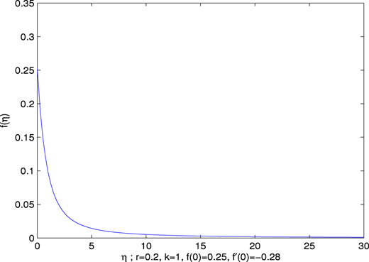
Figure 1 shows a typical solution to the Navier–Stokes equation (11) illustrating the above result. Another result can readily be obtained here for :
Proof. Under the hypotheses of the preceding theorem where for all , Eq. (13) will show that . This implies that it is not possible to have as . Nor is it possible to have a solution that reaches zero equilibrium at finite : when , for the same reason.
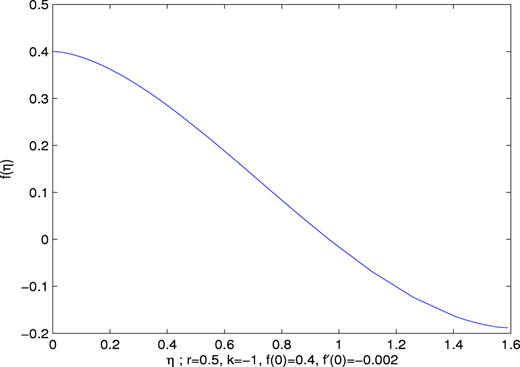
In fact, solutions where , will cross the axis, and will eventually terminate at some point where , for some finite . This can be illustrated with the aid of numerical integrators. (See Figure 2.)
3.1 The case
As for the case where , we begin by showing that a solution exists where at some finite : observe that with we have , so that Eq. (13) yields:
Choose small enough in absolute value so that:
This choice will show that a solution exists such that for some , we have , and the solution terminates. It can readily be verified that , within the interval of the given solution, so that the above arguments stay valid.
On the other hand, there exists a solution which crosses the axis at some finite . This can be established using the same arguments in the proof of the preceding theorem, as was stated earlier. However, observe that since and , we must have
in order to avoid any inflection point (with , and since the solution will cross the axis once it has an inflection point, as the curvature will continue to be negative once it is negative). Observe, now, that inequality (18) implies , and therefore , where is a constant, and for . Now, if where , then the above inequality for holds, but inequality (13) will have a divergent term on the right-hand side, and therefore will reach zero in finite time say , with , so that conditions (12) will not be satisfied. On the other hand, if we let , with (of order less than , is real and ) then the above inequality still holds, but again a contradiction occurs upon substituting into (11), where we are led again to obtaining an inflection point. Therefore:
The dynamics here is the following: Solutions exist where reaches zero at some , and for all , for some large enough . However, there exists a certain value for where further reduction of the initial condition (increase in absolute value of the gradient) shall yield a solution that crosses the horizontal axis ( does not reach zero but rather stays negative). This happens since the decay of solutions (changes in and ) becomes extremely slow with proportional to (namely observe the factor with and where now ), allowing the non-autonomous term with the presence of , to exceed the last term , of the governing equation (11). This leads to a change in curvature, and therefore solutions will cross the axis, and will not satisfy from (12). This is verified by numerical integrators, and is illustrated in Figure 3: In particular the two upper curves reach a point where (11) is undefined with . Such solutions reach a terminal point, that they cannot be extended beyond. The solution in the bottom illustrates that there is a minimum for with those terminal points, after which solutions change curvature, and eventually will cross the axis.
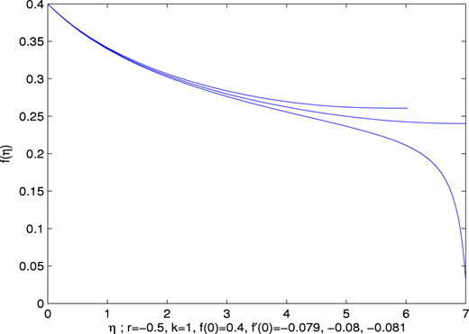
A set of solutions to Eq. (11) with . They do not satisfy (12): There is a minimum for where reaches zero and (11) becomes undefined (a terminal point), beyond which solutions change curvature with on the entire solution domain.
3.2 The case
Unlike some of the previous cases, observe that in this case the governing equation (11) implies that . In fact, the curvature stays negative for some interval say , until drops in value while becomes more negative (see (11)). Then becomes positive, and it can readily be established that stays positive, on the infinite interval, if is large enough. Additionally, if the solution crosses the horizontal axis then will continue to be positive in this case of , and in fact if the solution does cross the axis it will eventually terminate with : once the solution attains a negative value, say , then we have , so that , which implies that will reach zero at finite . With the existence of solutions that cross the axis and then reach , as stated by the remarks given above, another result is needed:
Lemma 4. Two different solutions of (11) with the same initial f(0), but two different initial gradients , do not intersect for any . Furthermore, if with , then for all .
Proof. Given a solution with say , take another solution with , and where . The two solutions will be different in, at least a small interval say , and on that interval. If the two solutions intersect, then would be the same for and at the point of intersection, and therefore the right-hand side of (13) would be larger for the solution . This, in turn, implies that is larger than in absolute value, so that at the point of intersection, and now this is a contradiction (which in fact can also be illustrated geometrically, as well as analytically).
Now, using the continuity with respect to initial conditions, it can be concluded that the solution with the larger initial absolute gradient will always have a larger , at all where (i.e. avoiding a situation where ). Otherwise, at an where , let us say that represents the difference between the two solutions: . Then, observe that we would have , where is larger precisely by the amount (see (11)). Now we can take small enough so that the two solutions would intersect at some point, say at (an argument here can be made, for example, using a Taylor series expansion). This contradicts the first result in the lemma, proven above. Now, note that the possibility would imply that at some , since . Therefore, the obtained contradiction would still eliminate this last possibility. This result can be generalized using similar arguments for .
With solutions that reach constant , and the above lemma, we may “construct” a solution that reaches zero equilibrium () at finite : given a solution that reaches equilibrium at a constant , take another solution with a smaller so that it reaches a terminal point , at a smaller value of (with ). (This is a consequence of the preceding lemma.) Proceed in this fashion to find a solution that reaches zero at finite (See Figure 4). Another way to view this is the following: we have solutions that cross the horizontal axis at with a negative , so that taking another solution with a smaller leads to a less negative at , and with . If the change in is small enough, the new solution will then cross the axis, but at a larger and with a smaller (at the point of crossing). This process can be continued until the required solution is reached. So this solution is established here, mathematically, as a limiting case.
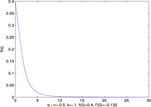
A typical solution to Eq. (11) with . It reaches zero equilibrium at finite ( ≈ in this particular figure).
A typical solution to Eq. (11) with . It reaches zero equilibrium at finite ( ≈ in this particular figure).
Remark. Observe that the two different views above involve the same set of solutions.
In fact, analysis of Eq. (13) suggests that other solutions may exist but where for all , and with possibly an infinite number of points where the solution changes curvature. In such a case, the quantity does not approach zero due to balancing positive and negative terms in (13), which cannot approach zero. Furthermore, it can be easily checked that any solution of (11), with , and any choice of , will satisfy for all as long as , and cannot approach an equilibrium .
4. Conclusions
We studied a reduced problem from the Navier–Stokes and the continuity equations in two-dimensional Cartesian coordinates, with Eulerian description, for incompressible non-Newtonian fluids. We have shown the existence of positive solutions to the reduced ODE, , , and where . Such solutions exist if . Those solutions may not be unique if the flow behavior index . On the other hand, positive solutions do not exist if . Additionally, a solution exists and has been explicitly expressed when .
Dongming Wei is supported by the Kazakhstan Ministry of Education Grant # AP05134166. The publisher wishes to inform readers that the article “Existence of self-similar solutions of the two-dimensional Navier–Stokes equation for non-Newtonian fluids” was originally published by the previous publisher of the Arab Journal of Mathematical Sciences and the pagination of this article has been subsequently changed. There has been no change to the content of the article. This change was necessary for the journal to transition from the previous publisher to the new one. The publisher sincerely apologises for any inconvenience caused. To access and cite this article, please use Wei, D., Al-Ashhab, S. (2019), “Existence of self-similar solutions of the two-dimensional Navier–Stokes equation for non-Newtonian fluids”, Arab Journal of Mathematical Sciences, Vol. 26 No. 1/2, pp. 167-178. The original publication date for this paper was 20/04/2019.

