

We consider the kernel-based classifier proposed by Younso (2017). This nonparametric classifier allows for the classification of missing spatially dependent data. The weak consistency of the classifier has been studied by Younso (2017). The purpose of this paper is to establish strong consistency of this classifier under mild conditions. The classifier is discussed in a multi-class case. The results are illustrated with simulation studies and real applications.
1. Introduction
In many applications one needs to classify spatial data that have been collected incompletely. The classification of incomplete-data problem, in which certain features are missing from particular feature vectors, exists in a wide range of fields, including image labeling, computer vision and others. For example, in the remote sensing technology, because of the internal malfunction of satellite sensors and poor atmospheric conditions such as thick cloud, the acquired remote sensing images often suffer from missing information at certain pixels and one wants to classify these pixels using the information in the nearest identified pixels. Many existing classification algorithms assume either certain parametric distributions for the data or certain forms of separating curves or surfaces. These parametric classifiers are suboptimal and of limited use in practical applications where little information about the underlying distributions is available a priori. In comparison, nonparametric classifiers are usually more flexible in accommodating different data structures, and are hence more desirable. [21] has proposed a nonparametric approach allowing to include contextual features for classifying missing spatial data and has investigated the consistency of the classifier under mild conditions. In nonparametric spatial estimation, the existing works concern mainly the estimation of a probability density and regression functions, see the key references: [2–4,15] and [14]. More recently, [5] has proposed a kernel spatial density estimator allowing for the analysis of spatial clustering. In this work, we establish strong consistency of the classifier proposed by [21] and then, we check its performance with simulation studies and applications. We consider a strictly stationary random field defined on some probability space and taking values in , for some integer . In the problem of classification, for each , is a vector of features and is the label (class) of . A point will be referred to as a site. For , we define the rectangular region by . We will write if . Define and assume that the random field is observed on a subset with is a bounded set for large enough. When processing a particular site, its features are not used at all, but only the features of its neighbors will be considered. In other words, we wish to predict the label of a new site based only on observations in a vicinity, say , where the set is not containing . Let , where is a fixed bounded set of sites not containing with ( is also the cardinal of each ). We assume that is a random vector taking values in with , and that the components of are ordered according to an arbitrary order on indices, for example the lexicographic order. The pair may be completely described by , the probability measure for , and , the regression of on . Assume that for each , has the same distribution as the pair . We will create a classifier mapping into the predicted label of . The error rate, or risk, of a rule is . This is minimized by the rule
whose error rate is called the Bayes-optimal risk and is called the Bayes rule. Clearly, predicts the label of the site using only , the value of , while the features vector does not affect the classification procedure at all. This means that well work event if is completely missing. Unfortunately, we cannot use (1.1) directly because it depends on the distribution of which is generally unknown. So, we take and we use the training data to construct a classifier . We consider the classifier obtained by extending the classifier of [21] to the multi-class case as follows:
where denotes the indicator of the set , the kernel is a density function on , and is a sequence of bandwidths tending to zero as tends to infinity. In one hand, the sum in (1.2) is taken over instead of just to ensure that always exists and that the sums make sense. On the other hand, for each new site , the classifier predicts the missing label independently of its features vector which does not belong neither to the training sample nor to the components set of . Consequently, may classify even if its own features vector is completely missing and that makes our method exhibit good performance in comparison with the classical spatial Markovian model. [6] proposes a nonparametric approach to extend the result of [2] to the non-Markovian case by using two kernels in the estimator in order to control both the distance between observations and that between spatial locations without using a specific vicinity for the non-observed site. This latter approach may be developed to classify spatial data but it does not work when one wants to classify sites with missing or incomplete features. Let be the error probability of . Generally, we cannot hope to design a classifier that achieve the Bayes error probability but it is possible that the limit behavior of compares favorably to . This idea is encapsulated in the notion of consistency.
The classifier is called weakly consistent if
Since is bounded, the weak consistency of is equivalent to the convergence of towards in probability which means that strong consistency implies the weak consistency.
In this paper, we investigate the strong consistency of under some mild mixing conditions.
2. Notation and general hypotheses
Let be a probability space and let and be two sub -fields of . The -mixing coefficient between and is defined by
and the -mixing coefficient is defined by
Let be a random field on (Ω and taking values in some space (Ω′).
The random field is called strongly mixing if there exists with as , and for any with finite cardinals,
The -mixing condition is one of the most popular mixing conditions. This condition is satisfied by many spatial models. Examples can be found in [17,19] and [11].
The random field is called -mixing if there exists with as , and for any with finite cardinals,
is a regular kernel, that is, there exist and such that , where is the closed ball of radius and center at .
For each , has a density with respect to Lebesgue measure and for each with , has a density such that , for some .
The random field is -mixing and there exists such that .
Assumption 1 is used by [8] and [7] in the i.i.d. case. It may be satisfied if where is a non-negative and decreasing function on and is the Euclidean norm. Hence, the Gaussian kernel is regular. Assumption 2, used by [21] to prove the weak consistency, is similar to that used by [3]. It is satisfied for example if and are uniformly bounded. Assumption 3 means that the random field is arithmetically -mixing which implies that it is also strongly mixing with since .
3. Preliminary lemmas
This section is a collection of technical lemmas which will be used to prove the strong consistency result stated in Theorem 4.1. Let denote the -norm for any real . The following lemma is a direct consequence of the covariance inequality of Ibragimov [12] and the inequality .
If , and are strictly positive reals such that and and are two -valued random variables such that and , then
For any sub -fields and of , we denote by the -field generated by . The following coupling lemma of Berbee [1] will be needed to establish the asymptotic results.
Let be a random variable on (Ω with values in some Polish space Ω′ and a sub -field of . Assume that there exists a random variable uniformly distributed over , independent of . Then, there exists a random variable measurable with respect to , distributed as and independent of , such that
We recall that a Polish space Ω′ is a topological space which is separable and completely metrizable (see [13]) and that most of the familiar objects of study in analysis involve Polish spaces. For example, for each integer , is Polish with the usual topology and , for all , is Polish with discrete topology. We also recall that a countable product of Polish spaces is Polish.
The following covering lemma can be found in [8].
Let for some , with and being small positive numbers such that . If Assumption 3 holds for some , then for any ,
For each , , where is the diameter of .
4. Main result
The weak consistency of the classifier (1.2) has been established by [21]. In this section we study the strong consistency of (1.2). The following theorem states the strong consistency under mild conditions.
Note that the assumption on the bandwidth, using by [21] to prove the weak consistency, is similar to the classical assumption used by [7] and [8] in the independent case. In addition, the condition on is minimal compared to that used by [4] and [3] since they have studied the rate of uniform convergence for the estimators. However, the restrictive constraints on the bandwidth in [4] and [3] are related to and one has to let in order to attain the classical assumption.
5. Simulation study including comparison with the classical kernel rule
Our aim in this section is to look at how the classifier (1.2) behaves on simulated samples by comparing it with the classical kernel rule. We use the R statistical programming environment to run a simulation study for . Let be the field of interest and suppose that the simulated data are observed on the area . Let
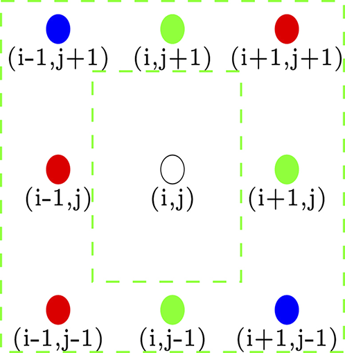
where is the set of non-observed sites which need to be classified. In this particular case, the vicinity of any missing site may be taken as in Figure 1.
It is important to note that the vicinity may be designed depending on the location of the missing site (see some typical examples in Figure 2) and that samples with larger size give more freedom to design vicinities.
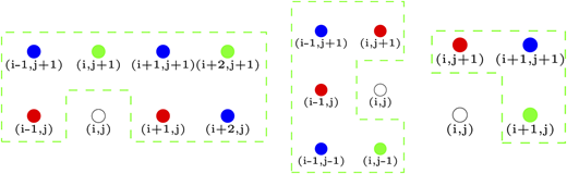
Three typical vicinities corresponding to three missing sites in different locations.
Three typical vicinities corresponding to three missing sites in different locations.
Figure 2 shows some examples of vicinities that can be used when the missing sites are not completely surrounded by already labeled sites (located at the edges of for example).
We suppose that the simulated fields have the covariance function
We use the classifier (1.2) with for where is the standard Gaussian density (Gaussian kernel). We suppose that are observations of a Gaussian mixture model:
with and . In order to illustrate the fact that our method works for multi-class, the data set is partitioned in three clusters as follows:
For each , we generate samples on the region with , , , and . In each replication, we use the classifier (1.2), constructed on the basis of the training data observed on , to re-predict the labels of sites in the test set . Figure 3 displays one replication for .
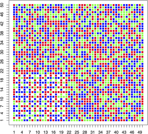
The training sites are colored in red (), green () or blue () and the sites to classify are blank.
The training sites are colored in red (), green () or blue () and the sites to classify are blank.
The optimal bandwidth is obtained by minimizing the cross-validation criterion on a training sample and the misclassification error rate () is evaluated based on the associated test sample. The average error rate () is obtained by averaging the error rates associated with the corresponding test samples.
Table 1 shows that the estimated optimal bandwidth and the average error rate decrease when the training sample size increases. This means that the practical results in the simulation study are in line with the theoretical results. Now, let us compare the average error rate () resulting from application of the proposed classifier with that resulting from application of the classical kernel rule.
5.1 Comparison with the classical kernel rule
The classical kernel rule is given, for any unlabeled site with , by
where is a kernel on (the Gaussian kernel is considered here), and is a sequence of bandwidths. In order for the classical kernel classifier to be usable in our case, we have to adjust it slightly by taking the sum over instead of , , for each with ,
From the theoretical point of view, this is justified by the fact that has the same asymptotic behavior on as on since is bounded. In this classical kernel method, we consider knowing the features vector of each element of and we use , the value of , to predict its class while we needed only observations in nearby sites to predict the label of by the classifier (1.2). We apply the classical kernel classifier to re-classify the elements of using the same training samples generated above and taking into account all the replications for each size . Similar to what we have done in application of (1.2), the optimal bandwidth is chosen by minimizing the cross-validation criterion on a training sample and the misclassification error rate () is evaluated based on the associated test sample. Table 2 reports the average error rate (AER), obtained by averaging the error rates associated with the corresponding test samples.
Estimated optimal bandwidths and average error rates corresponding to the classical kernel classifier with samples of different sizes.
| 25 | 50 | 80 | |
|---|---|---|---|
| 1.85 | 1.72 | 1.69 | |
| 23.4% | 18.7% | 13.2% |
By comparing Tables 1 and 2, we observe that the corresponding error values in the two tables begin to be close as increases. This supports the possibility of using the classifier (1.2) as an alternative to the classical kernel classifier when we have to classify sites with missing features.
6. Application to a real data
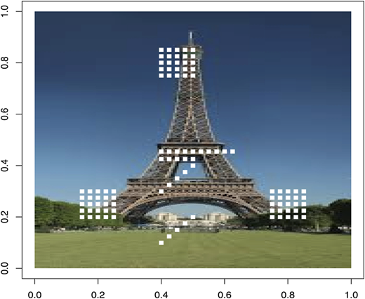
A digital image is nothing than data numbers indicating variation of , and () at a particular location on a grid of pixels. An color value is specified with: . Each parameter defines the intensity of the color as an integer between and . For example, is rendered as blue, because the blue parameter is set to its highest value and the others are set to . One can divide color values by in order to provide values in the interval . Let us have an image of Eiffel tower with missing pixels as in Figure 3.
We use the R package to convert a image into -d array of numbers. The package offers the function which can read raster graphics (consisting of “pixel matrices”) in format into . It returns either a single matrix with gray values in or -d array with the values in , say . In our example of Figure 3, the dimensions of are . Thus, the elements of represent the intensities of the color , for , at all pixels of the grid . For example, the matrix displays the intensities of in each pixel of the region:
Le where is the intensity of the color at the pixel . Since our purpose is to classify new sites with completely missing features, we set an arbitrary threshold of 0.4 and we define labels as follow:
The set of missing pixels is taken as a test set, say . We use the classifier (1.2) (see (1.7) for the binary version) to classify each element of based on its eight-neighbors. The optimal bandwidth is evaluated by minimizing the cross-validation criterion on the known sites where we get . The misclassification error rate () is evaluated on where we obtain which indicates that there are only four misclassified cases out of classified cases (see Figure 4).
Now let us use the support vector machine (S V M) classifier to re-classify the elements of . In this case we should suppose that the RGB value is known for each element of . For implementing support vector machine in R programming language, we use the package . According to this classifier, we get a misclassification error of and this permits to conclude that our kernel classifier in this example proceeds well compared to the (SVM) procedure.
7. Proof of Theorem 4.1
Without loss of generality, we prove the theorem in the binary case where takes values in since no additional argument is required to prove it in the multi-class case. However, the Bayes classifier (1.1) in the binary case is given by
and the classifier (1.2) is given by
Define
Consequently, the classifier (7.1) can be written as
By Theorem 2.3 in [7], the consistency will be proved if we show that
But
Hence, in order to prove (7.1), it suffices to show that
and
The proof of (7.3) is the same as in the i.i.d. case (see [7], pp. 156–157 ). So, it suffices to prove (7.4). To do that, we will employ the blocking technique used in [4]. Let for some (where stands for the integer part). Without loss of generality, we suppose that there exists a positive integer such that for each . Let
We define blocks as follow, for each ,
As a consequence, we have , and for each , and for any . Let , for each and . Hence, for a fixed , we have for any , and
Let be a set of independent and identically distributed random vectors such that they are independent of and is identically distributed with . In order to make sense to the blocking technique, we define random vectors as follow: for each ,
It is clear that and . Now, for a fixed and each , let be a vector whose components are ordered according to a given order on indices. Applying Lemma 3.2 together with the blocks decomposition introduced by [10] (see also [20]) on the family of vectors , we can generate independent copies such that: they are mutually independent, and for each , has the same distribution as . Furthermore, by Lemma 3.5, we have since for large enough. Thus, the two vectors and are independent for each and with . Now, for each , there exists such that . Since for each , denote , for each (or ). As a consequence
By (7.5), we can write
If we denote
then
where is the constant defined in Lemma 3.3. Since is bounded and as , so for large enough. Therefore, we get
for some generic positive constant . Since , by Borel–Cantelli lemma, we have
with probability one. Now, we will show that
Consequently, in order to establish (7.10), it is sufficient to show that
for each . Without loss of generality, we show (7.12) for . If the elements of are enumerated in an arbitrary manner, we can write with . Denote , for each , where the components of are ordered according to an arbitrary order on indices. Recall that for and suppose that is replaced by if where . Hence, by the blocks decomposition, the random vectors are independent. Let be a real function defined as follows
For where and for each , using Lemma 3.3, we have
Hence, since with , by McDiarmid’s inequality [16], we have for every ,
Since with , then and Borel–Cantelli lemma yields
As a consequence
with probability one. In order to complete the proof of (7.12) for , it remains to show that
The proof of (7.14) can be achieved by the same arguments used by ([21], Section 5), in addition to benefiting from Lemmas 3.1, 3.4 and 3.5. Combining (7.9), (7.10), (7.12)–(7.14), we get (7.4). Finally, (7.3) and (7.4) yield (7.2) and the proof is completed. □
The author would like to thank the anonymous referees whose valuable comments led to an improved version of the paper. The publisher wishes to inform readers that the article “Strong consistency of a kernel-based rule for spatially dependent data” was originally published by the previous publisher of the Arab Journal of Mathematical Sciences and the pagination of this article has been subsequently changed. There has been no change to the content of the article. This change was necessary for the journal to transition from the previous publisher to the new one. The publisher sincerely apologises for any inconvenience caused. To access and cite this article, please use “Younso, A., Kanaya, Z., Azhari, N. (2019), “Strong consistency of a kernel-based rule for spatially dependent data”, Arab Journal of Mathematical Sciences, Vol. 26 No. 1/2, pp. 211-225. The original publication date for this paper was 13/11/2019.
