Infinite horizon impulse control problem with jumps and continuous switching costs

Amami, Rim; Pontier, Monique; Abidi, Hani

doi:10.1108/AJMS-10-2020-0088

Purpose

The purpose of this paper is to show the existence results for adapted solutions of infinite horizon doubly reflected backward stochastic differential equations with jumps. These results are applied to get the existence of an optimal impulse control strategy for an infinite horizon impulse control problem.

Design/methodology/approach

The main methods used to achieve the objectives of this paper are the properties of the Snell envelope which reduce the problem of impulse control to the existence of a pair of right continuous left limited processes. Some numerical results are provided to show the main results.

Findings

In this paper, the authors found the existence of a couple of processes via the notion of doubly reflected backward stochastic differential equation to prove the existence of an optimal strategy which maximizes the expected profit of a firm in an infinite horizon problem with jumps.

Originality/value

In this paper, the authors found new tools in stochastic analysis. They extend to the infinite horizon case the results of doubly reflected backward stochastic differential equations with jumps. Then the authors prove the existence of processes using Envelope Snell to find an optimal strategy of our control problem.

1. Introduction

The main motivation of this paper is to prove the existence of an optimal strategy which maximizes the expected profit of a firm in an infinite horizon problem with jumps. More precisely, let a Brownian motion ${(W_{t})}_{t \geq 0}$ and an independent Poisson measure $μ (d t, d e)$ defined on a probability space $(Ω, A, ℙ)$ and let $F$ be the right continuous complete filtration generated by the pair $(W, μ)$ ⁠. Assume that a firm decides at stopping times to change its technology to determine its maximum profit. Let ${1, 2}$ be the possible technologies set. A right continuous left limited stochastic process X models the firm log value and a process $(ξ_{t}, t \geq 0)$ taking its values in ${1, 2}$ models the state of the chosen technology. The firm net profit is represented by a function f, the switching technology costs are represented by $c_{1,2}$ and $c_{2,1}, β > 0$ is a discount coefficient. Then, the problem is to find an increasing sequence of stopping times $\hat{α} : = {(\hat{τ_{n}})}_{n \geq - 1},$ where ${\hat{τ}}_{- 1} = 0,$ optimal for the following impulse control problem

K (\hat{α}, i, x) : = \underset{α \in A}{ess \sup} E_{i, x} [\int_{0}^{+ \infty} e^{- β s} f (ξ_{s}, X_{s}) d s - \sum_{n \geq 0} {e^{- β τ_{2 n}} c_{1,2} + e^{- β τ_{2 n + 1}} c_{2,1}}],

where $A$ denotes the set of admissible strategies. The Snell envelope tools show that the problem reduces to the existence of a pair of right continuous left limited processes $(Y^{1}, Y^{2})$ ⁠. This idea originates from Hamadène and Jeanblanc [1]. Their results are extended to infinite horizon case and mixed processes (namely jump-diffusion with a Brownian motion and a Poisson measure). In [1] the authors considered a power station which has two modes: operating and closed. This is an impulse control problem with switching technology without jump of the state variable. They solved the starting and stopping problem when the dynamics of the system are the ones of general adapted stochastic processes.

The existence of $(Y^{1}, Y^{2})$ is established via the notion of doubly reflected backward stochastic differential equation. In this context, another interest of our work is to extend to the infinite horizon case the results of doubly reflected backward stochastic differential equations with jumps. Specifically, a solution for the doubly reflected backward stochastic differential equation associated to a stochastic coefficient $g,$ a null terminal value and a lower (resp. an upper) barrier ${(L_{t})}_{t \geq 0} (resp . {(U_{t})}_{t \geq 0})$ is a quintuplet of $F$ -progressively measurable processes ${(Y_{t}, Z_{t}, V_{t}, K_{t}^{+}, K_{t}^{-})}_{t \geq 0}$ which satisfies

{\begin{array}{l} Y_{t} = \int_{t}^{+ \infty} e^{- β s} g (s) d s + \int_{t}^{+ \infty} d K_{s}^{+} - \int_{t}^{+ \infty} d K_{s}^{-} - \int_{t}^{+ \infty} Z_{s} d W_{s} - \int_{t}^{\infty} \int_{E} V_{s} (e) \tilde{μ} (d s, d e), \\ L_{t} \leq Y_{t} \leq U_{t}, \forall t \geq 0 \\ \int_{0}^{t} (Y_{s} - L_{s}) d K_{s}^{+} = \int_{0}^{t} (Y_{s} - U_{s}) d K_{s}^{-} = 0, ℙ - a . s . \end{array}

(1)

where $\tilde{μ}$ is the compensated measure of $μ .$

Another specificity of this paper is to promote a constructive method of the solution of a BSDEs with two barriers. Specifically, we do not assume the so called Mokobodski's hypothesis. Indeed this one is not so easy to check (see e.g. [2] in finite horizon and continuous case). Our assumptions are more natural and easy to check on the barriers in practical cases.

The notion of backward stochastic differential equation (BSDE) was studied by Pardoux and Peng [3] (meaning in such a case $L = - \infty, U = + \infty$ and $K^{\pm} = 0$ ⁠). To our knowledge, they were the first to prove the existence and uniqueness of adapted solutions, under suitable square-integrability and Lipschitz-type condition assumptions on the coefficients and on the terminal condition. Several authors have been attracted by this area that they applied in many fields such as Finance [1, 4–6], stochastic games and optimal control [7–10], and partial differential equations [11].

The existence and the uniqueness of BSDE solutions with two reflecting barriers and without jumps have been first studied by Cvitanic and Karatzas [4] (generalization of El Karoui et al. [5]) applied in Finance area by El Karoui et al. [6]. There is a lot of contributions on this subject since then, consisting essentially in weakening the assumptions, adding jumps and considering an infinite horizon.

The extension to the case of BSDEs with one reflecting barrier and jumps has been studied by Hamadène and Ouknine [8] considering a finite horizon $T = 1$ ⁠. The authors show the existence and uniqueness of the solution using the penalization scheme and the Snell envelope tools. They stress the connection between such reflected BSDEs and integro-differential mixed stochastic optimal control. The authors' assumptions are: the terminal value is a square integrable random variable, the drift coefficient function $g (t, ω, y, z, v)$ is uniformly Lipschitz with respect to $(y, z, v)$ and the obstacle ${(S_{t})}_{t \leq 1}$ is a right continuous left limited process whose jumps are totally inaccessible. Hamadène and Ouknine [12] deal with reflected BSDEs in finite horizon, the barrier being right continuous left limited and progressively measurable. Hamadène and Hassani [9] proved existence and uniqueness results of local and global solutions for doubly reflected BSDEs driven by a Brownian motion and an independent Poisson measure in finite horizon. The authors applied these results to solve the related zero-sum Dynkin game.

Here the model is inspired from the papers [5, 8–10, 12]. But their results do not apply directly to the situation which here requires an infinite horizon. Moreover we connect the reflected BSDE with the impulse control problem. All these papers provide a solution to the reflected BSDE problem which are here extended to the case of infinite horizon by adding a discount coefficient and imposing admissibility conditions of strategies. In this paper, the drift function is assumed to be Lipschitz and non-increasing in $y .$ It is proved that the reflected BSDE solutions are limit of Cauchy sequences in appropriate complete metric spaces. Another interesting area is the one of oblique reflections, meaning a multimodal switching problem, see for instance [13–15]. El Asri [14] considers the same problem proposed by Hamadène and Jeanblanc [1] and extends it to the infinite horizon case without jump of the state variable, namely a power station which produces electricity and has several modes of production (the lower, the middle and the intensive modes). Naturally, the switching from one mode to another induces costs. The optimal switching problem is solved by means of probabilistic tools such as the Snell envelop of processes and reflected backward stochastic differential equations. Moreover their proofs are based on the verification theorem and the system of variational inequalities that we do not use.

Our purpose is similar to the one in [16], but instead of using Snell envelope and fixed point theorem as they do, here the two barriers case is solved using comparison theorem in one barrier case and adding some assumptions on the drift coefficient g.

This paper is composed of six sections. Section 2 presents the impulse control problem and describes the corresponding model. Section 3 introduces a pair of right continuous left limited processes $(Y^{1}, Y^{2})$ that allows one to exhibit an optimal strategy. Section 4 extends the doubly reflected BSDEs tools in the infinite horizon setting with jumps: first the case of a single barrier with general Lipschitz drift is solved, then a comparison theorem is proved, finally the uniqueness and the existence of solution for the doubly reflected BSDE under suitable assumptions are proved in case of drift non depending on state $(y, z, v)$ ⁠. Section 5 proves the existence of the required pair $(Y^{1}, Y^{2})$ ⁠, and provides an application of these doubly reflected BSDE to a switching problem. Finally, with some simulations, the results allow to define an optimal strategy in Section 6. An appendix is devoted to an extension of Gronwall's lemma and some technical results.

2. Preliminaries and problem formulation

Let $(Ω, F, ℙ)$ be a filtered complete probability space with a right continuous complete filtration $F = {(F_{t})}_{t \geq 0},$ generated by the two following mutually independent processes:

$a 1 -$ dimensional Brownian motion $W = {(W_{t})}_{t \geq 0} .$
a point process $N_{t} : = \int_{0}^{t} \int_{E} e μ (d s, d e)$ associated with a Poisson random measure μ on $ℝ^{+} \times E,$ where $E = ℝ \ {0},$ for some $m \geq 1$ endowed with its Borel σ-algebra $ℰ$ ⁠, with compensator $ν (d t, d e) = d t λ (d e),$ for a σ-finite measure λ on $(E, ℰ), \int_{E} (1 \land {| e |}^{2}) λ (d e) < \infty;$ $\tilde{μ} : = μ - ν$ denotes the compensated measure associated with $μ .$

Assume that a firm decides at random times to switch the technology in order to maximize its profit: the firm switches from the technology 1 to the technology 2 along a sequence of stopping times. An impulse control strategy is defined as a sequence $α : = {(τ_{n})}_{n \geq - 1},$ where ${(τ_{n})}_{n \geq - 1}$ is a sequence increasing to infinity of $F$ -stopping times with $τ_{- 1} = 0$ ⁠. The sequence $(τ_{n})$ models the impulse time sequence of the system as follows: for every $n \geq 0, τ_{2 n}$ is the time when the firm moves from technology 1 to technology 2 and $τ_{2 n + 1}$ is the time when the firm goes from 2 to 1. A càdlàg process $(ξ_{t})$ taking its values in ${1, 2}$ is defined by

ξ_{t} : = \sum_{n \geq 0} 1_{[τ_{2 n - 1}, τ_{2 n} [} (t) + 2 \sum_{n \geq 0} 1_{[τ_{2 n}, τ_{2 n + 1} [} (t) .

(2)

Given $K > 0$ and a measurable map $γ : ℝ \times E \to ℝ$ such that

\sup_{e \in E} | γ (0, e) | \leq K and \sup_{e \in E} | γ (x, e) - γ (x^{'}, e) | \leq K | x - x^{'} | \forall x, x^{'} \in ℝ,

(3)

the firm value is defined as $S_{t} : = \exp X_{t}, t \geq 0,$ where $(X_{t})$ is the càdlàg process

X_{t} : = X_{0} + \int_{0}^{t} b (X_{s}) d s + \int_{0}^{t} σ (X_{s}) d W_{s} + \int_{0}^{t} \int_{E} γ (X_{s^{-}}, e) \tilde{μ} (d s, d e),

(4)

where $X_{0} \in ℝ$ is the initial condition, $b : ℝ \to ℝ$ and $σ : ℝ \to ℝ$ are two measurable functions satisfying the K-Lipschitz condition (thus the sublinear growth condition).

The instantaneous net profit of the firm is given in terms of a positive function f, depending on the technology in use and the value of the firm. Let $c_{2,1}$ and $c_{1,2}$ be the positive switching technology costs, $c_{i, j}$ if one passes from technology i to technology $j,$ with regular enough assumptions which will be specified later. One considers a discount coefficient $β > 0$ then, the profit associated with a strategy α is defined as

k (α) : = \int_{0}^{+ \infty} e^{- β s} f (ξ_{s}, X_{s}) d s - \sum_{n \geq 0} {e^{- β τ_{2 n}} c_{1,2} + e^{- β τ_{2 n + 1}} c_{2,1}},

and the expected profit of the firm is defined by

K (α, i, x) : = E_{i, x} [\int_{0}^{+ \infty} e^{- β s} f (ξ_{s}, X_{s}) d s - \sum_{n \geq 0} {e^{- β τ_{2 n}} c_{1,2} + e^{- β τ_{2 n + 1}} c_{2,1}}] .

(5)

Definition 2.1.

The strategy $α : = {(τ_{n})}_{n \geq - 1}$ is admissible if:

\int_{0}^{+ \infty} e^{- β s} f (ξ_{s}, X_{s}) d s and \sum_{n \geq 0} {e^{- β τ_{2 n}} c_{1,2} + e^{- β τ_{2 n + 1}} c_{2,1}}

belong to $L^{1} (Ω, F_{\infty}, ℙ) .$ We denote by $A$ the set of admissible strategies.

Here, the impulse control problem is to prove the existence of an admissible strategy $\hat{α}$ which maximizes the expected profit:

K (\hat{α}, i, x) : = \sup_{α \in A} E_{i, x} [\int_{0}^{+ \infty} e^{- β s} f (ξ_{s}, X_{s}) d s - \sum_{n \geq 0} {e^{- β τ_{2 n}} c_{1,2} + e^{- β τ_{2 n + 1}} c_{2,1}}] .

(6)

The following notations will be used:

$T : = {θ : F - stopping time}, T_{t} : = {θ \in T : θ \geq t} .$
$P : = {F - progressively measurable càdlàg processes} .$
$C^{2} : = {{(X_{t})}_{t \geq 0} \in P : such that E [\sup_{t \geq 0} {| X_{t} |}^{2}] < \infty} .$
$ℍ^{1} : = {{(X_{t})}_{t \geq 0} \in P : such that E [\sqrt{\int_{0}^{\infty} {| X_{t} |}^{2} d t}] < \infty} .$
$ℍ^{2} : = {{(X_{t})}_{t \geq 0} \in P : such that E [\int_{0}^{\infty} {| X_{t} |}^{2} d t] < \infty} .$
$P^{d}$ the σ algebra of $F$ -predictable sets on $Ω \times [0, + \infty [.$
$L^{2} : {V : Ω \times [0, + \infty] \times E \to ℝ, P^{d} \otimes ℰ - measurable s . t . E [\int_{0}^{\infty} \int_{E} {| V_{s} (e) |}^{2} λ (d e) d s] < \infty}$
$L^{p} : = L^{p} (Ω, F_{\infty}, ℙ), p = 1, 2.$
$ℍ^{p} : = ℍ^{p} (Ω, F_{\infty}, ℙ), p = 1, 2.$
Class [D] : ${processes U : (U_{θ}, θ \in T) uniformly integrable} .$

3. The impulse control problem

Section 5 shows that the problem reduces to the existence of a pair of càdlàg processes $(Y^{1}, Y^{2})$ using the Snell envelope tools: this idea originates from Hamadène and Jeanblanc [1]. The existence of $(Y^{1}, Y^{2})$ is established in Section 5 via the reflected BSDEs tools. Indeed, the solution of the reflected BSDE corresponds to the value function of an optimal stochastic control problem and these processes allow to build an optimal switching strategy. We based on [17] to use the fundamental optimal control concepts.

Proposition 3.1.

Assume that there exist two right continuous left limited, regular (meaning that the predictable projection coincide with the left limit) $ℝ$ -valued processes $Y^{1} = {(Y_{t}^{1})}_{t \geq 0}$ and $Y^{2} = {(Y_{t}^{2})}_{t \geq 0}$ of class [D] and satisfying the properties

Y_{t}^{1} = \underset{θ \in T_{t}}{ess \sup} E [\int_{t}^{θ} e^{- β s} f (1, X_{s}) d s - e^{- β θ} c_{1,2} + Y_{θ}^{2} | F_{t}]

(7)

\begin{array}{l} Y_{t}^{2} = \underset{θ \in T_{t}}{ess \sup} E [\int_{t}^{θ} e^{- β s} f (2, X_{s}) d s - e^{- β θ} c_{2,1} + Y_{θ}^{1} | F_{t}] \\ Y_{\infty}^{1} = Y_{\infty}^{2} = 0, c_{i, j} > 0. \end{array}

(8)

where $f (i, .)$ are positive functions satisfying $\int_{0}^{\infty} e^{- β s} f^{2} (i, X_{s}) d s \in L^{1}, i = 1, 2$ ⁠. Then $Y_{0}^{1} = \sup_{α \in A} K (α, 1, x) .$ Moreover, the strategy $\hat{α} = {(τ_{n})}_{n \geq 0}$ defined as follows:

\begin{array}{l} τ_{- 1} : = 0 \\ τ_{2 n} : = \inf {t > τ_{2 n - 1}, Y_{t}^{1} \leq - e^{- β t} c_{1,2} + Y_{t}^{2}}, \forall n \geq 0 \\ τ_{2 n + 1} : = \inf {t > τ_{2 n}, Y_{t}^{2} \leq - e^{- β t} c_{2,1} + Y_{t}^{1}} \end{array}

is optimal for the impulse control problem (6).

The proof is based on the properties of the Snell envelope. The scheme of the proof is similar to the one in [18] and also [14, Appendix A, p. 246] as soon as the processes $Y^{i}$ are regular. As a consequence of (7) and (8), remark that almost surely

- e^{- β t} c_{1,2} \leq Y_{t}^{1} - Y_{t}^{2} \leq e^{- β t} c_{2,1} .

(9)

4. Reflected BSDE with jumps and infinite horizon

In this section, the results from [10] are extended to infinite horizon reflected backward stochastic differential equations with general jumps, showing existence and uniqueness of an infinite horizon solution, imposing additional assumptions on the drift function and using appropriate estimates of the process Y. The following assumptions are done:

$(H_{1}) :$ A map $g : Ω \times [0, + \infty [\times ℝ^{1 + d} \times L^{2} (E, ℰ, λ; ℝ) \to ℝ$ which is $F$ -progressively measurable and:

{\begin{array}{l} \forall (t, z, v), y \mapsto g (t, y, z, v) is non increasing almost surely, \\ \exists C > 0 such that for any t \geq 0, y, y^{'} \in ℝ, z, z^{'} \in ℝ^{d}, v, v^{'} \in L^{2} (E, ℰ, λ; ℝ) : \\ | g (t, y, z, v) - g (t, y^{'}, z^{'}, v^{'}) | \leq C (| y - y^{'} | + | z - z^{'} | + | | v - v^{'} | |) a . s . \end{array}

where the norm of $L^{2} (E, ℰ, λ; ℝ)$ is defined as ${‖ v ‖}^{2} : = \int_{E} v^{2} (e) λ (d e) .$

$(H_{1}^{'})$ ⁠: An $F$ -progressively measurable map $g : Ω \times [0, + \infty [\to ℝ$ such that $\int_{0}^{\infty} e^{- β s} g^{2} (s) d s \in L^{1},$
$(H_{2}) :$ Let the barriers ${(L_{t})}_{t \geq 0}$ and ${(U_{t})}_{t \geq 0}$ be $F$ -progressively measurable continuous real valued processes satisfying

E [\sup_{t \geq 0} {(L_{t}^{+})}^{2}] < \infty, \lim_{t \to + \infty} \sup L_{t} \leq 0 \leq U_{t}, ℙ a . s .

To prove the existence of the solution for doubly reflected BSDE with jumps and infinite horizon, we first consider the case of a single barrier (Section 4.1) then a comparison theorem is proved in Section 4.2.

4.1 Reflected BSDE in case of a single barrier, infinite horizon

In this subsection, the case of infinite horizon reflected BSDE with one barrier and general jumps is considered.

Definition 4.1.

Let $(e^{- β .} g, L)$ be given. A solution of the reflected BSDE associated to $(e^{- β .} g, L)$ is a quadruplet of processes $(Y, Z, V, K)$ satisfying for any $t \geq 0$ ⁠:

$Y \in C^{2}$ ⁠, $Z \in ℍ^{2}$ and $V \in L^{2}$ ⁠,
almost surely

Y_{t} = \int_{t}^{+ \infty} e^{- β s} g (s, Y_{s}, Z_{s}, V_{s}) d s + \int_{t}^{+ \infty} d K_{s} - \int_{t}^{+ \infty} Z_{s} d W_{s} - \int_{t}^{\infty} \int_{E} V_{s} (e) \tilde{μ} (d s, d e),

(10)

(3)
almost surely $L_{t} \leq Y_{t},$
(4)
$(K_{t})$ is a non-decreasing process satisfying $E [{(\int_{0}^{\infty} d K_{s})}^{2}] < \infty, K_{0} = 0,$ and for any t

\int_{0}^{t} (Y_{s -} - L_{s}) d K_{s} = 0, ℙ- a . s .

We then prove the following:

Theorem 4.2.

Let $(e^{- β .} g, L)$ satisfy Hypotheses $(H_{i}), i = 1, 2$ ⁠. Then there exists a unique process $(Y, Z, K, V)$ solution to the BSDE associated to $(e^{- β .} g, L)$ ⁠.

Proof: (1) As a first step, the uniqueness of the solution is insured: if there exist two solutions, the proof of uniqueness is a standard one. For instance, look at Theorem 4.8 proof.

(2)
Under the hypothesis $E [\sup_{t} {(L_{t})}^{2}] < \infty,$ Theorem 2.1 [10] can be applied: there exists a quadruplet $(Y^{T}, Z^{T}, K^{T}, V^{T})$ verifying $Y^{T} \in C^{2}, Z^{T} \in ℍ^{2}, V^{T} \in L^{2},$ (actually restricted to $t \in [0, T]$ ⁠) and $\forall t \leq T :$

\begin{array}{l} L_{t} \leq Y_{t}^{T}, \\ Y_{t}^{T} = \int_{t}^{T} e^{- β s} g (s, Y_{s}^{T}, Z_{s}^{T}, V_{s}^{T}) d s + \int_{t}^{T} d K_{s}^{T} - \int_{t}^{T} Z_{s}^{T} d W_{s} - \int_{t}^{T} \int_{E} V_{s}^{T} (e) \tilde{μ} (d s, d e), \end{array}

(11)

E {(\int_{0}^{T} d K_{s}^{T})}^{2} < \infty; \forall t \geq 0, \int_{0}^{t} (Y_{s^{-}}^{T} - L_{s^{-}}) d K_{s}^{T} = 0 ℙ a . s .

(12)

Considering $T \leq S, S, T \in ℝ^{+},$ one has $\forall s \leq T :$

\begin{array}{l} d (Y_{s}^{S} - Y_{s}^{T}) = - e^{- β s} [g (s, Y_{s}^{S}, Z_{s}^{S}, V_{s}^{S}) - g (s, Y_{s}^{T}, Z_{s}^{T}, V_{s}^{T})] d s \\ - [d K_{s}^{S} - d K_{s}^{T}] + [Z_{s}^{S} - Z_{s}^{T}] d W_{s} + \int_{E} [V_{s}^{S} (e) - V_{s}^{T} (e)] \tilde{μ} (d s, d e) . \end{array}

(13)

Applying Itô's formula to the process $s \to {(Y_{s}^{S} - Y_{s}^{T})}^{2}$ between t and T yields

\begin{array}{l} {(Y_{T}^{S})}^{2} = {(Y_{t}^{S} - Y_{t}^{T})}^{2} + \int_{t}^{T} {(Z_{s}^{S} - Z_{s}^{T})}^{2} d s + \sum_{t < s \leq T} {[Δ_{s} (Y^{T} - Y^{S})]}^{2} \\ - 2 \int_{t}^{T} e^{- β s} (Y_{s}^{S} - Y_{s}^{T}) [g (s, Y_{s}^{S}, Z_{s}^{S}, V_{s}^{S}) - g (s, Y_{s}^{T}, Z_{s}^{T}, V_{s}^{T})] d s \\ + 2 \int_{t}^{T} (Y_{s}^{S} - Y_{s}^{T}) [Z_{s}^{S} - Z_{s}^{T}] d W_{s} + 2 \int_{t}^{T} \int_{E} [(Y_{s -}^{S} - Y_{s -}^{T}) \\ (V_{s}^{S} (e) - V_{s}^{T} (e))] \tilde{μ} (d s, d e) \\ - 2 \int_{t}^{T} (Y_{s -}^{S} - L_{s} + L_{s} - Y_{s -}^{T}) (d K_{s}^{S} - d K_{s}^{T}) . \end{array}

(14)

Using $(Y_{s}^{S} - L_{s}) d K_{s}^{S} = (Y_{s -}^{T} - L_{s}) d K_{s}^{T} = 0$ and $L_{s} \leq Y_{s}^{S}$ and $Y_{s}^{T},$ one has

\int_{t}^{T} (Y_{s -}^{S} - L_{s} + L_{s} - Y_{s -}^{T}) (d K_{s}^{S} - d K_{s}^{T}) = \int_{t}^{T} [(L_{s} - Y_{s -}^{S}) d K_{s}^{T} + (L_{s} - Y_{s -}^{T}) d K_{s}^{S}] \leq 0,

so we get

\begin{array}{l} {(Y_{t}^{S} - Y_{t}^{T})}^{2} + \int_{t}^{T} {(Z_{s}^{S} - Z_{s}^{T})}^{2} d s + \sum_{t < s \leq T} {[Δ_{s} (Y^{T} - Y^{S})]}^{2} \\ \leq {(Y_{T}^{S})}^{2} + 2 \int_{t}^{T} e^{- β s} (Y_{s}^{S} - Y_{s}^{T}) [g (s, Y_{s}^{S}, Z_{s}^{S}, V_{s}^{S}) - g (s, Y_{s}^{T}, Z_{s}^{T}, V_{s}^{T})] d s \\ - 2 \int_{t}^{T} (Y_{s}^{S} - Y_{s}^{T}) [Z_{s}^{S} - Z_{s}^{T}] d W_{s} - 2 \int_{t}^{T} \int_{E} [(Y_{s -}^{S} - Y_{s -}^{T}) (V_{s}^{S} (e) - V_{s}^{T} (e))] \tilde{μ} (d s, d e) . \end{array}

(15)

Considering the decomposition: $g (s, Y_{s}^{S}, Z_{s}^{S}, V_{s}^{S}) - g (s, Y_{s}^{T}, Z_{s}^{T}, V_{s}^{T}) = g (s, Y_{s}^{S}, Z_{s}^{S}, V_{s}^{S}) - g (s, Y_{s}^{T}, Z_{s}^{S}, V_{s}^{S}) + g (s, Y_{s}^{T}, Z_{s}^{S}, V_{s}^{S}) - g (s, Y_{s}^{T}, Z_{s}^{T}, V_{s}^{S}) + g (s, Y_{s}^{T}, Z_{s}^{T}, V_{s}^{S}) - g (s, Y_{s}^{T}, Z_{s}^{T}, V_{s}^{T}),$ the Lipschitz property of the function g, the Cauchy-Schwarz inequality and the non-increasing property of the map $y \mapsto g (t, y, z, v)$ for any $(t, z, v)$ and $α > 0$ lead to

\begin{array}{l} 2 \int_{t}^{T} e^{- β s} (Y_{s}^{S} - Y_{s}^{T}) [g (s, Y_{s}^{S}, Z_{s}^{S}, V_{s}^{S}) - g (s, Y_{s}^{T}, Z_{s}^{T}, V_{s}^{T})] d s \\ \leq 2 C \int_{t}^{T} e^{- β s} | Y_{s}^{S} - Y_{s}^{T} | [| Z_{s}^{S} - Z_{s}^{T} | + ‖ V_{s}^{S} - V_{s}^{T} ‖] d s \\ \leq 2 C α \int_{t}^{T} e^{- β s} {| Y_{s}^{S} - Y_{s}^{T} |}^{2} d s + \frac{C}{α} \int_{t}^{T} {| Z_{s}^{S} - Z_{s}^{T} |}^{2} d s + \frac{C}{α} \int_{t}^{T} \int_{E} {| V_{s}^{S} (e) - V_{s}^{T} (e) |}^{2} λ (d e) d s . \end{array}

Thus for any $α > 0 :$

\begin{array}{l} {(Y_{t}^{S} - Y_{t}^{T})}^{2} + \int_{t}^{T} {(Z_{s}^{S} - Z_{s}^{T})}^{2} d s + \sum_{t < s \leq T} {[Δ_{s} (Y^{T} - Y^{S})]}^{2} \\ \leq {(Y_{T}^{S})}^{2} + 2 C α \int_{t}^{T} e^{- β s} {| Y_{s}^{S} - Y_{s}^{T} |}^{2} d s + \frac{C}{α} \int_{t}^{T} {| Z_{s}^{S} - Z_{s}^{T} |}^{2} d s \\ + \frac{C}{α} \int_{t}^{T} \int_{E} {| V_{s}^{S} (e) - V_{s}^{T} (e) |}^{2} λ (d e) d s \\ - 2 \int_{t}^{T} (Y_{s}^{S} - Y_{s}^{T}) [Z_{s}^{S} - Z_{s}^{T}] d W_{s} - 2 \int_{t}^{T} \int_{E} [(Y_{s -}^{S} - Y_{s -}^{T}) (V_{s}^{S} (e) - V_{s}^{T} (e))] \tilde{μ} (d s, d e) . \end{array}

(16)

Remark that $Δ_{s} (Y^{T} - Y^{S})$ includes the jumps of the Poisson measure μ. So

E [\sum_{t < s \leq T} {[Δ_{s} (Y^{T} - Y^{S})]}^{2}] = E [\int_{t}^{T} \int_{E} {(V_{s}^{T} (e) - V_{s}^{S} (e))}^{2} λ (d e) d s] .

(17)

Then, since $Y^{S}, Y^{T} \in C^{2}, Z^{S}, Z^{T} \in ℍ^{2}$ and $V^{S}, V^{T} \in L^{2},$ the third line in (16) is a martingale; thus taking the expectation of both sides with $α = 2 C$ yields for any $t \leq T$

\begin{array}{l} E {(Y_{t}^{S} - Y_{t}^{T})}^{2} \leq \\ E {(Y_{t}^{S} - Y_{t}^{T})}^{2} + \frac{1}{2} \int_{t}^{T} E {(Z_{s}^{S} - Z_{s}^{T})}^{2} d s + \frac{1}{2} E \int_{t}^{T} \int_{E} {| V_{s}^{S} (e) - V_{s}^{T} (e) |}^{2} λ (d e) d s \\ \leq E {(Y_{T}^{S})}^{2} + 4 C^{2} E \int_{t}^{T} e^{- β s} {| Y_{s}^{S} - Y_{s}^{T} |}^{2} d s . \end{array}

(18)

On the one hand, Lemma 7.2 , we obtain for any $ε > 0,$ T and any S:

E {(Y_{T}^{S})}^{2} \leq \exp (\frac{4 C^{2} + 2 C + 1}{β}) ϕ (T),

(19)

where $ϕ (T) : = \frac{1}{β} ∥ g ∥^{2} e^{- β T} + \frac{1}{ε} E \sup_{s \geq T} {(L_{s}^{+})}^{2} + ε E {(\int_{T}^{S} d K_{s}^{S})}^{2}$ as defined in (61). Using Gronwall's lemma, inequality (19) becomes

E {(Y_{t}^{S} - Y_{t}^{T})}^{2} \leq ϕ (T) \exp (\frac{2 C^{2} + 2 C + 1}{β}) \exp (\frac{2 C^{2}}{β}) .

On the other hand, we have

\int_{T}^{S} d K_{s}^{S} = Y_{T}^{S} - \int_{T}^{S} e^{- β s} f (s, Y_{s}^{S}, Z_{s}^{S}, V_{s}^{S}) d s + \int_{T}^{S} Z_{s}^{S} d W_{s} + \int_{T}^{S} V_{s}^{S} \tilde{μ} (d s, d e),

and from the Lipschitz property, we get

\int_{T}^{S} e^{- β s} f (s, Y_{s}, Z_{s}) d s \leq C \int_{T}^{S} e^{- β s} (| Y_{s}^{S} | + | Z_{s}^{S} | + | | V_{s}^{S} | |) d s + \int_{T}^{S} e^{- β s} f (s, 0, 0, 0) d s .

Using estimation (19), there exists a constant M, such that for any $T, S :$

\frac{1}{4} E {(\int_{T}^{S} d K_{s}^{S})}^{2} \leq M ϕ (T) + \frac{1}{β} {| | f | |}^{2} e^{- β T} .

If we subtract from $ϕ (T)$ the term $ε E {(\int_{T}^{S} d K_{s}^{S})}^{2}$ we get

(\frac{1}{4} - ε M) E {(\int_{T}^{S} d K_{s}^{S})}^{2} \leq (1 + M) \frac{1}{β} | | f^{2} | | e^{- β T} + \frac{M}{ε} E sup_{s \geq T} {(L_{s}^{+})}^{2} .

(20)

This implies that the expectation on the left tends to zero uniformly when $ε$ is chosen small enough: indeed, since ${sup}_{s} L_{s}^{+} \in L^{2},$ by Lebesgue's monotone convergence $E \sup_{s \geq T} {(L_{s}^{+})}^{2}$ tends to 0 when T tends to infinity. Globally $ϕ (T) \to 0$ when T tends to infinity and we obtain using (19) that the sequence $(Y^{T})$ is a Cauchy sequence which converges in $L^{2} (Ω)$ to the process $Y$ ⁠. Thus Lemma 7.2 concludes that, t being fixed, $(Y_{t}^{T}, T \geq t)$ is a Cauchy sequence in $L^{2} (Ω, F_{t}, ℙ)$ ⁠, its limit defines the $F_{t}$ -measurable random variable $Y (t, .) .$ It is a family of random variables. We later prove that actually the limit Y is a process.

(3)
Turning to Z and V, to deal with the convergence in $ℍ^{2}$ respectively in $L^{2}$ ⁠, An argument similar to (63) shows that the sequence $(Z^{T})$ is a Cauchy sequence in $ℍ^{2}$ ⁠, its limit defines a process Z which belongs to $ℍ^{2}$ and $(V^{T})$ is a Cauchy sequence in $L^{2}$ ⁠, its limit defines a process V which belongs to $L^{2}$ ⁠.
(4)
We now prove that there exists a process $Y \in C^{2}$ which is the limit of a Cauchy sequence in $C^{2}$ ⁠.
(a) Coming back to (16), for all $α > 0,$ we get
$\begin{array}{l} \sup_{t \leq T} {(Y_{t}^{S} - Y_{t}^{T})}^{2} \\ \leq {(Y_{T}^{S})}^{2} + C α \sup_{s \leq T} {| Y_{s}^{S} - Y_{s}^{T} |}^{2} \frac{1}{β} + \frac{C}{α} \int_{0}^{T} {| Z_{s}^{S} - Z_{s}^{T} |}^{2} d s + \frac{C}{α} \int_{0}^{T} \int_{E} {| V_{s}^{S} (e) - V_{s}^{T} (e) |}^{2} λ (d e) d s \\ + 2 \sup_{t \leq T} | \int_{t}^{T} (Y_{s}^{S} - Y_{s}^{T}) [Z_{s}^{S} - Z_{s}^{T}] d W_{s} | \\ + 2 \sup_{t \leq T} | \int_{t}^{T} \int_{E} [(Y_{s–}^{S} - Y_{s–}^{T}) (V_{s}^{S} (e) - V_{s}^{T} (e))] \overline{μ} (d s, d e) | . \end{array}$

The Burkholder-Gundy-Davis inequality gives the existence of a constant $C_{1} > 0$ such that

\begin{array}{l} 2 E sup_{t \leq T} | \int_{t}^{T} (Y_{s}^{S} - Y_{s}^{T}) [Z_{s}^{S} - Z_{s}^{T}] d W_{s} | \leq 2 C_{1} E {(\int_{0}^{T} {[Y_{s}^{S} - Y_{s}^{T}]}^{2} {[Z_{s}^{S} - Z_{s}^{T}]}^{2} d s)}^{1 / 2} \\ \leq 2 C_{1} E sup_{s \leq T} | Y_{s}^{S} - Y_{s}^{T} | {(\int_{0}^{T} {[Z_{s}^{S} - Z_{s}^{T}]}^{2} d s)}^{1 / 2} \\ \leq C_{1} [γ E sup_{s \leq T} {| Y_{s}^{S} - Y_{s}^{T} |}^{2} + \frac{1}{γ} E (\int_{0}^{T} {[Z_{s}^{S} - Z_{s}^{T}]}^{2} d s)], \end{array}

for all $γ > 0$ ⁠. Similarly

E [sup_{t \leq T} | \int_{t}^{T} \int_{E} [(Y_{s -}^{S} - Y_{s -}^{T}) (V_{s}^{S} (e) - V_{s}^{T} (e))] \tilde{μ} (d s, d e) |] \leq C_{1} [γ E sup_{s \leq T} {| Y_{s}^{S} - Y_{s}^{T} |}^{2} + \frac{1}{γ} \int_{0}^{T} \int_{E} E [{(V_{s}^{S} (e) - V_{s}^{T} (e))}^{2}] λ (d e) d s] .

Gathering these bounds yields

\begin{array}{l} (1 - \frac{C α}{β} - 2 C_{1} γ) [E sup_{s \leq T} {(Y_{s}^{S} - Y_{s}^{T})}^{2}] \\ \leq E {(Y_{T}^{S})}^{2}] + \frac{C}{α} \int_{0}^{T} {| Z_{s}^{S} - Z_{s}^{T} |}^{2} d s + \frac{C}{α} \int_{0}^{T} \int_{E} {| V_{s}^{S} (e) - V_{s}^{T} (e) |}^{2} λ (d e) d s \\ + \frac{C_{1}}{γ} [E (\int_{0}^{T} {[Z_{s}^{S} - Z_{s}^{T}]}^{2} d s) + \int_{0}^{T} \int_{E} E [{(V_{s}^{S} (e) - V_{s}^{T} (e))}^{2}] λ (d e) d s] . \end{array}

(21)

Choosing $α$ and $γ$ such that $1 - \frac{C α}{β} - 2 C_{1} γ > 0,$ using Lemma 7.2 and the facts that $(Z^{T}, T \geq t)$ is a Cauchy sequence in $ℍ^{2}$ ⁠, and $(V^{T}, T \geq t)$ is a Cauchy sequence in $L^{2}$ ⁠, then $E [{sup}_{t \leq T} {(Y_{t}^{S} - Y_{t}^{T})}^{2}]$ goes to 0 when S and T go to infinity.

(5)
Now one proves the other items of the proposition: Item (2) According to (4.1) for all $t_{1} < t_{2} \leq T$

\int_{t_{1}}^{t_{2}} d K_{s}^{T} = Y_{t_{2}}^{T} - Y_{t_{1}}^{T} - \int_{t_{1}}^{t_{2}} e^{- β s} g (s, Y_{s}^{T}, Z_{s}^{T}, V_{s}^{T}) d s + \int_{t_{1}}^{t_{2}} Z_{s}^{T} d W_{s} + \int_{t_{1}}^{t_{2}} \int_{E} V_{s}^{T} (e) \tilde{μ} (d s, d e),

(22)

and due to the almost sure convergence of a subsequence of $(Y^{T}, Z^{T}, V^{T})$ and the continuity of the function g, the right hand side of Eqn (22) converges almost surely.

Thus $\int_{t_{1}}^{t_{2}} d K_{s}$ is defined as the $L^{2}$ and almost sure limit of the right hand side of (22). Hence, for almost sure limit, we get the reflected BSDE (10).

Item (3) For any $T \geq t,$ one has $L_{t} \leq Y_{t}^{T}$ ⁠, and using almost convergence of a subsequence, one deduces Item (3).

Item (4) The $L^{2}$ convergence in (22) proves that $\int_{t}^{\infty} d K_{s} \in L^{2} .$ Moreover, for all T using (12), we get:

(Y_{s -}^{T} - L_{s}) d K_{s}^{T} = 0.

(23)

On the one hand, for fixed $(ω, t) \in Ω \times [0, T]$ the left continuous and right limited function $s \to Y_{s -} - L_{s}$ is the uniform limit on $[0, t]$ of a sequence $(f^{k} (ω), k)$ of step functions:

lim_{k} sup_{0 \leq s \leq t} | f_{s}^{k} (ω) - (Y_{s -} - L_{s}) | = 0.

We now deal with the successive bounds

| \int_{0}^{t} (Y_{s -} - L_{s}) d K_{s}^{T} - \int_{0}^{t} (Y_{s -} - L_{s}) d K_{s} | \leq \int_{0}^{t} | Y_{s -} - L_{s} - f_{s}^{k} | d K_{s}^{T} + | \int_{0}^{t} f_{s}^{k} d K_{s}^{T} - \int_{0}^{t} f_{s}^{k} d K_{s} | + \int_{0}^{t} | Y_{s -} - L_{s} - f_{s}^{k} | d K_{s} .

(24)

For $(ω, t)$ fixed above, for any $ε > 0$ there exists $N (ω, t)$ such that

\forall k \geq N, sup_{0 \leq s \leq t} | f_{s}^{k} (ω) - (Y_{s -} - L_{s}) | \leq ε,

so the first and third terms in (24) are bounded

\int_{0}^{t} | Y_{s -} - L_{s} - f_{s}^{k} | d K_{s}^{T} + \int_{0}^{t} | Y_{s -} - L_{s} - f_{s}^{k} | d K_{s}^{T} \leq ε (K_{t}^{T} + K_{t}) .

(25)

Remark that ${lim}_{T \to \infty} (K_{t}^{T} + K_{t}) (ω) = 2 ε K_{t} (ω) .$

We now fix $k \geq N (ω, t),$ and we remark that for any step function $h :$

\int_{0}^{t} h (s) d K_{s}^{T} \to_{T \to \infty} \int_{0}^{t} h (s) d K_{s} .

Thus when T goes to infinity the second term in (24) satisfies

| \int_{0}^{t} f_{s}^{k} d K_{s}^{T} - \int_{0}^{t} f_{s}^{k} d K_{s} | \to 0.

(26)

For any $ε$ ⁠, using (25) and (26) the limit of (24) when T goes to infinity is bounded by $2 ε K_{t} (ω) .$ This yields the fact that ${lim}_{T \to \infty} \int_{0}^{t} (Y_{s -} - L_{s}) d K_{s}^{T} = \int_{0}^{t} (Y_{s -} - L_{s}) d K_{s} .$

Finally using (23) we get

\int_{0}^{t} (Y_{s -} - L_{s}) d K_{s}^{T} = \int_{0}^{t} (Y_{s -} - L_{s}) d K_{s}^{T} - \int_{0}^{t} (Y_{s -}^{T} - L_{s}) d K_{s}^{T} = \int_{0}^{t} (Y_{s -} - Y_{s -}^{T}) d K_{s}^{T} .

Thus

| \int_{0}^{t} (Y_{s -} - L_{s}) d K_{s}^{T} | \leq sup_{0 \leq s \leq t} | Y_{s -} - Y_{s -}^{T} | | K_{t}^{T} |

which goes to 0 when T goes to infinity according to the convergence of $Y^{T}$ to Y in $C^{2}$ and of $K^{T}$ in $L^{2} .$ So the proof of (4) is done.

■

In case of a deterministic function g, meaning g is defined on $ℝ^{+} \times ℝ \times ℝ^{d}$ ⁠, an alternative proof of Theorem 4.3 (under the same hypotheses) can be provided using penalization method, as for instance Section 6 in [6] concerning continuous case, but here directed by a pair Brownian motion-Poisson measure. We associate to $(g_{k} (s, y, z) : = e^{- β s} g (s, y, z) + k {(y - L_{s})}^{-})$ where the function $g_{k}$ satisfies Assumption $(H_{1})$ ⁠, since $g_{k}$ is obviously non decreasing and uniformly Lipschitz, the solution $(Y^{k}, Z^{k}, V^{k})$ in $(C^{2}, ℍ^{2}, L^{2})$ of the following BSDE

Y_{t}^{k} = \int_{t}^{\infty} (e^{- β s} g (s, Y_{s}^{k}, Z_{s}^{k}) + k {(Y_{s}^{k} - L_{s})}^{-}) d s - \int_{t}^{\infty} Z_{s}^{k} d W_{s} - \int_{t}^{\infty} \int_{E} V_{s}^{k} (e) \tilde{μ} (d s, d e) .

(27)

Since $k \to g_{k}$ is non decreasing, the standard comparison theorem proves that actually, for any fixed t $(Y_{t}^{k})$ is a non-decreasing sequence in $L^{2}$ ⁠, so it is almost surely and in $L^{2}$ convergent to the random variable $Y_{t} : = {lim}_{k \to \infty} Y_{t}^{k} .$ Using similar arguments as those ones in (4.1) $(Y^{k})$ is a Cauchy sequence in $C^{2}$ so the limit defines the $C^{2}$ process $Y .$ Now it is standard [19] to prove the existence of a non decreasing process K such that

\int_{t}^{\infty} d K_{s} : = lim_{k \to \infty} \int_{t}^{\infty} k {(Y_{s}^{k} - L_{s})}^{-} d s,

and the existence of $Z, V \in (ℍ^{2}, L^{2})$ such that

Y_{t} = \int_{t}^{\infty} e^{- β s} g (s, Y_{s}, Z_{s}) d s + \int_{t}^{\infty} d K_{s} - \int_{t}^{\infty} Z_{s} d W_{s} - \int_{t}^{\infty} \int_{E} V_{s} (e) \tilde{μ} (d s, d e),

(28)

Y_{t} \geq L_{t} and \int_{t}^{\infty} Y_{s -} d K_{s} = \int_{t}^{\infty} L_{s} d K_{s} .

This alternative method allows us to prove the following result.

Proposition 4.3.

Under Hypotheses $(H_{1}^{'}, H_{i}, i = 2)$ ⁠, g being defined on $ℝ^{+} \times Ω,$ one has

Y_{t} = \underset{θ \in T_{t}}{ess sup} E [\int_{t}^{θ} e^{- β s} g (s) d s + L_{θ} 1_{{θ < \infty}} | F_{t}] .

(29)

Proof: The uniqueness of the solution (step (i) in the proof of Theorem 4.2) insures that this solution is the limit of the penalized Eqn (27): Y is the limit of the non-decreasing sequence $(Y^{k}) .$

Reproducing Step 2 in the proof of Theorem 3.1 [16] leads for any k to

Y_{t}^{k} = \underset{θ \in T_{t}}{ess sup} E [\int_{t}^{θ} e^{- β s} g (s) d s + Y_{θ}^{k} \land L_{θ} 1_{θ < \infty} | F_{t}],

so ${(Y_{t}^{k} + \int_{0}^{t} e^{- β s} g (s) d s)}_{t}$ is the Snell envelope of the process $J^{k} : t \to \int_{0}^{t} e^{- β s} g (s) d s + Y_{t}^{k} \land L_{t}$ which is increasing almost surely towards the process $J : t \to \int_{0}^{t} e^{- β s} g (s) d s + Y_{t} \land L_{t} .$ Remark that both $J^{k}$ and J are of class $[D]$ since both are uniformly bounded with $\int_{0}^{\infty} e^{- β s} | g (s) | d s + {sup}_{t} | L_{t} | \in L^{1} .$

Let us denote as $S N (Y)$ the Snell envelope of process Y. Then Lemma A.1 in Appendix [10, 12] allows to commute the increasing limit and the essential supremum: on the left hand side, $Y_{t}^{k} ↑ Y_{t}$ almost surely, on the right hand side $SN {(J^{k})}_{t} ↑ SN {(J)}_{t}$ which achieves the proof. ■

From now on, we consider a function g defined on $ℝ^{+} \times Ω$ satisfying Assumption $(H_{1}^{'}) .$

The following is an extension of Lemma 2.4 in [20]: in our case g is defined only on $ℝ^{+} \times Ω$ but the BSDE is directed by a mixed Brownian-Poisson process:

Lemma 4.4.

For $n \geq 0,$ let $({\overline{Y}}^{n}, {\overline{Z}}^{n}, {\overline{V}}^{n})$ be the solution of the single barrier reflected BSDE associated to the barrier $t \to - e^{- β t} | g (t) | - n {(y - U_{t})}^{+},$ where $U_{t} = c_{2,1} e^{- β t}$ and ${\overline{Y}}_{T}^{n} = 0, {sup}_{t} (L_{t}^{+}) \in L^{2}$ ⁠. Then almost surely for all $t \geq 0,$

n {({\overline{Y}}_{t}^{n} - U_{t})}^{+} \leq β c_{2,1} e^{- β t} .

Proof: The proof is similar to the one in [18].

The next step follows from Theorem 3.2 [20] or Proposition 4.12 [18].

Lemma 4.5.

Let $(ρ, θ, \tilde{V}, Π)$ be the solution of the reflected BSDE associated to the barriers L and $U : t \to - e^{- β t} | g (t) | - β c_{2,1} e^{- β t} .$ Then there exists a constant C such that

E [{(\int_{0}^{\infty} d Π_{s})}^{2}] \leq C,

(30)

and for all t : E [ρ_{t}^{2}] \leq C and E (\int_{t}^{\infty} θ_{s}^{2} d s) + E (\int_{t}^{\infty} \int_{E} {\tilde{V}}_{s}^{2} (e) λ (d e) d s) \leq C .

(31)

Proof: (1) By definition, we have

d ρ_{s} = (e^{- β s} | g (s) | - β c_{2,1} e^{- β s}) d s - d Π_{s} + θ_{s} d W_{s} + \int_{E} {\tilde{V}}_{s} (e) \tilde{μ} (d e, d s) .

Using Itô's formula, one has

E ({(ρ_{t})}^{2}) + E (\int_{t}^{\infty} θ_{s}^{2} d s) + E (\int_{t}^{\infty} \int_{E} {\tilde{V}}_{s}^{2} (e) λ (d e) d s) = 2 E [\int_{t}^{\infty} (- e^{- β s} | g (s) | - β c_{2,1} e^{- β t}) ρ_{s} d s] + 2 E [\int_{t}^{\infty} ρ_{s} d Π_{s}] .

(32)

The last term on the right hand side of (32) is bounded: for any $ε > 0$

2 E [\int_{t}^{\infty} ρ_{s} d Π_{s}] = 2 E [\int_{t}^{\infty} L_{s} d Π_{s}] \leq 2 E [sup_{s \geq t} | L_{s} | \int_{t}^{\infty} d Π_{s}] \leq \frac{1}{ε} E [{(sup_{s \geq t} | L_{s} |)}^{2}] + ε E [{(\int_{t}^{\infty} d Π_{s})}^{2}]

Gathering these bounds and using Assumption $(H_{1}^{'})$ yield

\begin{array}{l} E (ρ_{t}^{2}) + E (\int_{t}^{\infty} θ_{s}^{2} d s) + E (\int_{t}^{\infty} \int_{E} {\tilde{V}}_{s}^{2} (e) λ (d e) d s) \\ \leq E [\int_{t}^{\infty} (e^{- β s}) ρ_{s}^{2} d s] + E [\int_{t}^{\infty} [e^{- β s} {| g (s) |}^{2} + {(β c_{2,1})}^{2} e^{- β s}] d s] \\ + \frac{1}{ε} E [{(sup_{s \geq t} L_{s})}^{2}] + ε E [{(\int_{t}^{\infty} d Π_{s})}^{2}] . \end{array}

(33)

Let

φ (t) : = E [\int_{t}^{\infty} (e^{- β s} {| g (s) |}^{2} + {(β c_{2,1})}^{2} e^{- β s}) d s] + \frac{1}{ε} E [{(sup_{s \geq t} L_{s})}^{2}] .

Using extended Gronwall's Lemma 7.1 one has

E [{(ρ_{t})}^{2}] \leq (φ (t) + ε E [{(\int_{t}^{\infty} d Π_{s})}^{2}] \exp (\frac{1}{β}) .

(34)

Let us denote $ψ (t) : = φ (t) + ε E [{(\int_{t}^{\infty} d Π_{s})}^{2}],$ $ψ$ being a decreasing function.

(2)Coming back to (33) one has

E (\int_{t}^{\infty} θ_{s}^{2} d s) + E (\int_{t}^{\infty} \int_{E} {\tilde{V}}_{s}^{2} (e) λ (d e) d s) \leq E [\int_{t}^{\infty} (e^{- β s} + e^{- α s}) ρ_{s}^{2} d s] + ψ (t),

and from setting

γ = \frac{1}{β}

⁠:

E (\int_{t}^{\infty} θ_{s}^{2} d s) + E (\int_{t}^{\infty} \int_{E} {\tilde{V}}_{s}^{2} (e) λ (d e) d s) \leq \exp γ . \int_{t}^{\infty} (e^{- β s}) ψ (s) d s + ψ (t) \leq ψ (t) (1 + γ \exp γ) .

(35)

Now one turns to the estimate of

Π

⁠:

\int_{t}^{\infty} d Π_{s} = - ρ_{t} - \int_{t}^{\infty} (e^{- β s} | g (s) | + β c_{2,1} e^{- β s}) d s + \int_{t}^{\infty} θ_{s} d W_{s} + \int_{t}^{\infty} \int_{E} {\tilde{V}}_{s} (e) \tilde{μ} (d s, d e) .

So

\frac{1}{5} E {| \int_{t}^{\infty} d Π_{s} |}^{2} \leq E {| ρ_{t} |}^{2} + φ (t) + E \int_{t}^{\infty} θ_{s}^{2} d s + E \int_{t}^{\infty} \int_{E} {\tilde{V}}_{s}^{2} (e) λ (d e) d s .

Using and :

\frac{1}{5} E {| \int_{t}^{\infty} d Π_{s} |}^{2} \leq (φ (t) + ε E [{(\int_{t}^{\infty} d Π_{s})}^{2}]) (\exp γ + φ (t) + (1 + γ \exp γ)) .

This yields and , as soon as

ε

is chosen such that

1 > 5 ε (\exp γ + 1 + γ \exp γ) .

■

4.2 Comparison theorem in case of a single barrier

The following proposition is an extension of Theorem 2.2 in [10] to infinite horizon.

Proposition 4.6.

Assume that $(Y, Z, V, K)$ and $(Y^{'}, Z^{'}, V^{'}, K^{'})$ are solutions of the reflected BSDE with jumps (10) associated with $(g, L)$ and $(g^{'}, L)$ ⁠, satisfying Assumptions $(H_{i}, i = 1, 2),$ g being defined on $ℝ^{+} \times Ω \times ℝ \times ℝ^{d},$ $g^{'}$ being defined on $ℝ^{+} \times Ω \times ℝ \times ℝ^{d} \times L^{2},$ and assume in addition that

(H) : {ℙ almost surely \forall t : g (t, Y_{t}^{'}, Z_{t}^{'}) \leq g^{'} (t, Y_{t}^{'}, Z_{t}^{'}, V_{t}^{'}) .

Then, $Y_{t} \leq Y_{t}^{'}$ $ℙ$ -almost surely.

If moreover $g^{'}$ is defined on $ℝ^{+} \times Ω \times ℝ \times ℝ^{d},$ then $K_{t} \geq K_{t}^{'} t \geq 0, ℙ - p . s .$

Proof: Theorem 2.2 in [10] proves that for any $T,$ $ℙ -$ almost surely, $\forall t \leq T,$ $Y_{t}^{T} \leq Y_{t}^{' T}$ and in the case where $f^{'}$ does not depend on v, $d K_{t}^{T} \geq d K_{t}^{' T} .$

Theorem 4.2 proof gives us the almost sure convergence of $Y^{T}, K^{T}, Y'^{T}, K^{' T},$ so the inequalities are preserved when T goes to infinity.■

Here we summarize the results concerning the reflected BSDEs: In case of a function g defined on $ℝ^{+} \times Ω$ satisfying $(H_{1}^{'}),$ the functions

$t \to e^{- β t} g (t) - n {(y - U_{t})}^{+}, - e^{- β t} | g (t) | - n {(y - U_{t})}^{+}, - e^{- β t} | g (t) | - β c_{2,1} e^{- β s}$ satisfy Hypothesis $(H_{1})$ ⁠: Lipschitz property and non increasingness with respect to y.

The $F$ -progressively measurable process $({\overline{Y}}^{n}, {\overline{Z}}^{n}, {\overline{V}}^{n}, {\overline{K}}^{n})$ which is the unique solution of the reflected BSDE associated with $(- e^{- β t} | g (t) | - n {(y - U_{t})}^{+}, L)$ satisfies

{\overline{Y}}_{t}^{n} = - \int_{t}^{\infty} e^{- β s} | g (s) | d s - \int_{t}^{\infty} {\overline{Z}}_{s}^{n} d W_{s} - n \int_{t}^{\infty} {(Y_{s}^{n} - U_{s})}^{+} d s + \int_{t}^{\infty} d {\overline{K}}_{s}^{n} - \int_{t}^{\infty} \int_{E} {\overline{V}}_{s}^{n} (e) \tilde{μ} (d s, d e),

(36)

(2)
The $F$ -progressively measurable process $(ρ, θ, \tilde{V}, Π)$ which is the unique solution of the reflected BSDE associated with $(- e^{- β t} | g (t) | - E [{sup}_{s \geq t} | u_{s} | | F_{t}], L)$ satisfies

\begin{array}{l} ρ_{t} = - \int_{t}^{\infty} e^{- β s} | g (s) | d s - \int_{t}^{\infty} θ_{s} d W_{s} - \int_{t}^{\infty} β c_{2,1} e^{- β s} d s \\ + \int_{t}^{\infty} d Π_{s} - \int_{t}^{\infty} \int_{E} {\tilde{V}}_{s} (e) \tilde{μ} (d s, d e) . \end{array}

(37)

Thank to Lemma 4.4, one has the following inequalities:

e^{- β t} g (t) - n {({\overline{Y}}_{t}^{n} - U_{t})}^{+} \geq - e^{- β t} | g (t) | - n {({\overline{Y}}_{t}^{n} - U_{t})}^{+} \geq - e^{- β t} | g (t) | - β c_{2,1} e^{- β t} .

So as a consequence of Proposition 4.6, one has

Y^{n} \geq {\overline{Y}}^{n} \geq ρ; K^{n} \leq {\overline{K}}^{n} \leq Π,

(38)

where $Y^{n}$ and $K^{n}$ are introduced in (27). Finally, Lemma 4.5 proves that for all t and all $n,$

E [{(\int_{t}^{\infty} d K_{s}^{n})}^{2}] \leq C .

(39)

4.3 Double barrier reflected BSDE with jumps and infinite horizon

Now one considers the problem of reflection with respect to two barriers L and U in the case of drift g being defined on $ℝ^{+} \times Ω$ and satisfying $(H_{1}^{'})$ ⁠.

Definition 4.7.

Let $(e^{- β .} g, L, U)$ be given. A solution of the double reflected BSDE associated to $(e^{- β .} g, L, U)$ is a quintuplet of processes $(Y, Z, V, K^{+}, K^{-})$ satisfying for any $t \geq 0$ ⁠:

$Y \in C^{2}$ and $Z \in ℍ^{2}, V \in L^{2}$ ,
almost surely

\begin{array}{l} Y_{t} = \int_{t}^{+ \infty} e^{- β s} g (s) d s + \int_{t}^{+ \infty} d K_{s}^{+} - \int_{t}^{+ \infty} d K_{s}^{-} \\ - \int_{t}^{+ \infty} Z_{s} d W_{s} - \int_{t}^{\infty} \int_{E} V_{s} (e) \tilde{μ} (d s, d e) \end{array}

(40)

(3)
almost surely $L_{t} \leq Y_{t} \leq U_{t},$
(4)
$(K_{t}^{\pm})$ are non-decreasing processes satisfying $E [{(\int_{0}^{\infty} d K_{s}^{\pm})}^{2}] < \infty$ and for any t

\int_{0}^{t} (Y_{s -} - L_{s}) d K_{s}^{+} = \int_{0}^{t} (Y_{s -} - U_{s}) d K_{s}^{-} = 0, ℙ - a . s .

Theorem 4.8.

Let $(e^{- β .} g, L, U)$ satisfying Hypotheses $(H_{1}^{'}), (H_{2})$ ⁠, then there exists a unique solution $(Y, Z, K^{+}, K^{-}, V)$ to Eqn (4.7).

The proof is given in the following subsections.

4.3.1 Uniqueness of the solution

As a first result, one proves the uniqueness of solution when it exists.

proposition 4.9.

If there exists a solution of (40) satisfying Items (1) to (4), it is unique.

Proof: The proof of uniqueness is detailed, even if it is really standard, for stressing the role of the assumption $L_{s} < U_{s} .$ One assumes that there exist two solutions $(Y^{i}, Z^{i}, V^{i}, K^{\pm i}), i = 1, 2.$ Then they satisfy

d (Y_{s}^{1} - Y_{s}^{2}) = [Z_{s}^{1} - Z_{s}^{2}] d W_{s} - [d K_{s}^{+ 1} - d K_{s}^{+ 2}] + [d K_{s}^{- 1} - d K_{s}^{- 2}] - \int_{E} [V_{s}^{1} (e) - V_{s}^{2} (e)] \tilde{μ} (d s, d e) .

One has

\begin{array}{l} E {(Y_{t}^{1} - Y_{t}^{2})}^{2} + E [\int_{t}^{\infty} {(Z_{s}^{1} - Z_{s}^{2})}^{2} d s + \int_{t}^{\infty} \int_{E} {(V_{s}^{1} (e) - V_{s}^{2} (e))}^{2} λ (d e) d s] \\ \leq E [2 \int_{t}^{\infty} (Y_{s -}^{1} - L_{s} + L_{s} - Y_{s -}^{2}) (d K_{s}^{+ 1} - d K_{s}^{+ 2}) - 2 \int_{t}^{\infty} (Y_{s -}^{1} - U_{s} + U_{s} - Y_{s -}^{2}) (d K_{s}^{- 1} - d K_{s}^{- 2})] . \end{array}

Using Item (4) $(Y_{s -}^{i} - L_{s -}) d K_{s}^{+ i} = 0$ and $(Y_{s -}^{i} - U_{s -}) d K_{s}^{- i} = 0,$ the last line satisfies

E \int_{t}^{T} [- (Y_{s -}^{1} - L_{s}) d K_{s}^{+ 2} + (L_{s} - Y_{s -}^{2}) d K_{s}^{+ 1}] + E \int_{t}^{T} [(Y_{s -}^{1} - U_{s}) d K_{s}^{- 2} - (U_{s} - Y_{s -}^{2}) d K_{s}^{- 1}] \leq 0

(41)

since $L_{s} \leq Y_{s}^{i} \leq U_{s}$ ⁠.

It follows that for any t

E {(Y_{t}^{1} - Y_{t}^{2})}^{2} = \int_{t}^{\infty} E {(Z_{s}^{1} - Z_{s}^{2})}^{2} d s = E \int_{t}^{\infty} \int_{E} {| V_{s}^{1} (e) - V_{s}^{2} (e) |}^{2} λ (d e) d s = 0.

So $Y^{1} = Y^{2},$ $Z^{1} = Z^{2}$ ⁠, $V^{1} = V^{2}$ and as a consequence $K^{+ 1} - K^{- 1} = K^{+ 2} - K^{- 2} .$ Thus there exists a finite variation process $h = K^{+ 1} - K^{+ 2} = K^{- 1} - K^{- 2}$ satisfying $h (0) = 0,$ $(Y_{s -} - L_{s}) d h_{s} = 0$ and $(Y_{s -} - U_{s}) d h_{s} = 0.$ But the assumption $L_{s -} < U_{s -}$ contradicts these equalities if $h \neq 0$ : indeed as soon as $d h_{s} \neq 0,$ $(Y_{s -} - L_{s}) = 0$ and $(Y_{s -} - U_{s}) = 0$ so $L_{s}$ would be equal to $U_{s} .$ This concludes the proof of uniqueness.

4.3.2 Existence of the solution for double barrier reflected BSDE with jumps

Here one uses the so called penalization method: Let g satisfying $(H_{1}^{'})$ be the drift parameter and introduce $h (t, y) = e^{- β t} g (t) - n {(y - U_{t})}^{+}$ which obviously satisfies $(H_{1})$ ⁠.

So according to Theorem 4.2, Hypothesis (H2) still being in force, for each $n \in ℕ^{*},$ there exists a unique solution $(Y^{n}, Z^{n}, V^{n}, K^{n})$ of the reflected BSDE associated with $(e^{- β t} g (t, ω) - n {(y - U_{t})}^{+}, L)$ ⁠, meaning

\begin{array}{l} Y_{t}^{n} = \int_{t}^{\infty} e^{- β s} g (s) d s - \int_{t}^{\infty} Z_{s}^{n} d W_{s} - n \int_{t}^{\infty} {(Y_{s}^{n} - U_{s})}^{+} d s \\ + \int_{t}^{\infty} d K_{s}^{n} - \int_{t}^{\infty} \int_{E} V_{s}^{n} (e) \tilde{μ} (d s, d e) . \end{array}

(42)

From Proposition 4.6, the sequence $(Y^{n}, n \geq 1)$ (resp $K^{n}, n \geq 1$ ⁠) is non increasing (resp. non-decreasing), let us denote $Y, K^{+}$ their almost sure limits, consequence of monotonicity.

From the inequality $L_{t} \leq Y_{t} \leq Y_{t}^{1},$ it follows that $Y_{t} = {lim}_{n \to \infty} Y_{t}^{n}$ belongs to $L^{2}$ for all $t \in ℝ .$

The proof of Theorem 4.8 is done in five steps.

Step 1: There exists a constant $C \geq 0$ such that $\forall n \geq 0$ and $\forall t \geq 0,$ one has

E [{(Y_{t}^{n})}^{2} + {(- n \int_{t}^{\infty} {(Y_{s}^{n} - U_{s})}^{+} d s + \int_{t}^{\infty} d K_{s}^{n})}^{2} + \int_{t}^{\infty} {(Z_{s}^{n})}^{2} d s + \int_{t}^{\infty} \int_{E} {(V_{s}^{n} (e))}^{2} λ (d e) d s] \leq C .

Its formula yields

{(Y_{t}^{n})}^{2} + \int_{t}^{\infty} {| Z_{s}^{n} |}^{2} d s + \sum_{t < s} {[Δ_{s} (Y^{n})]}^{2} = + 2 \int_{t}^{\infty} e^{- β s} Y_{s}^{n} g (s) d s + 2 \int_{t}^{\infty} Y_{s -}^{n} d K_{s}^{n} - 2 n \int_{t}^{\infty} Y_{s}^{n} {(Y_{s}^{n} - U_{s})}^{+} d s - 2 \int_{t}^{\infty} Y_{s}^{n} Z_{s}^{n} d W_{s} - 2 \int_{t}^{T} \int_{E} (Y_{s -}^{n}) V_{s}^{n} (e) \tilde{μ} (d s, d e) .

(43)

By definition of the solution

\int_{t}^{\infty} Y_{s -}^{n} d K_{s}^{n} = \int_{t}^{\infty} L_{s} d K_{s}^{n} .

Then, since $L_{s} \leq Y_{s}^{n}, - Y_{s}^{n} \leq - L_{s} \Rightarrow - n Y_{s}^{n} {(Y_{s}^{n} - U_{s})}^{+} d s \leq - n L_{s} {(Y_{s}^{n} - U_{s})}^{+} d s$ , so $\forall t, \forall n :$

- n \int_{t}^{\infty} Y_{s}^{n} {(Y_{s}^{n} - U_{s})}^{+} d s \leq - \int_{t}^{\infty} L_{s} n {(Y_{s}^{n} - U_{s})}^{+} d s .

Thus, one has

\int_{t}^{\infty} Y_{s -}^{n} d K_{s}^{n} - n \int_{t}^{\infty} Y_{s}^{n} {(Y_{s}^{n} - U_{s})}^{+} d s \leq \int_{t}^{\infty} L_{s} (d K_{s}^{n} - n {(Y_{s}^{n} - U_{s})}^{+} d s) .

Using the Cauchy-Schwarz inequality, for any $ϵ > 0$ ⁠, one has for any t and n

2 \int_{t}^{\infty} L_{s -} (d K_{s}^{n} - {(n Y_{s}^{n} - U_{s})}^{+} d s) \leq ϵ {(\int_{t}^{\infty} (d K_{s}^{n} - n {(Y_{s}^{n} - U_{s})}^{+} d s)}^{2} + ϵ^{- 1} sup_{s \geq t} {(L_{s -})}^{2} .

On the other hand, with (38), Lemmas 4.4 and 4.5, for any t and n one has:

\begin{array}{l} {‖ \int_{t}^{\infty} (d K_{s}^{n} - n {(Y_{s}^{n} - U_{s})}^{+} d s) ‖}_{2} \leq {| | \int_{t}^{\infty} d K_{s}^{n} | |}_{2} + | | \int_{t}^{\infty} n {(Y_{s}^{n} - U_{s})}^{+} d s {| |}_{2} \\ \leq {| | \int_{t}^{\infty} d Π_{s} | |}_{2} + {| | \int_{t}^{\infty} e^{- β s} β c_{1,0} d s | |}_{2} < \infty . \end{array}

(44)

Similarly for any $c_{1} > 0$ one has

2 | \int_{t}^{\infty} e^{- β s} Y_{s}^{n} g (s) d s | \leq \int_{t}^{\infty} e^{- β s} {c_{1} {| Y_{s}^{n} |}^{2} + c_{1}^{- 1} {| g (s) |}^{2}} d s .

(45)

Note that the last line in the right hand side of (4.3) admits a zero expectation, and embedding the inequalities (44), (45) and (17) in the expectation of (4.3):

\begin{array}{l} E [{(Y_{t}^{n})}^{2} + \int_{t}^{\infty} {(Z_{s}^{n})}^{2} d s + \int_{t}^{\infty} \int_{E} {(V_{s}^{n} (e))}^{2} λ (d e) d s] \\ \leq E [c_{1} \int_{t}^{\infty} e^{- β s} {| Y_{s}^{n} |}^{2} d s + c_{1}^{- 1} \int_{t}^{\infty} e^{- β s} {| g (s) |}^{2} d s + ϵ {(k (t))}^{2} + ϵ^{- 1} \sup_{s \geq t} {(L_{s -})}^{2}], \end{array}

(46)

where k is the function defined as follows:

k (t) : = {| | \int_{t}^{\infty} d Π_{s} | |}_{2} + | | \int_{t}^{\infty} E [e^{- β s} β c_{1,0}] d s {| |}_{2} < \infty .

So one has

\begin{array}{l} E [{(Y_{t}^{n})}^{2} + \int_{t}^{\infty} {(Z_{s}^{n})}^{2} d s + \int_{t}^{\infty} \int_{E} {(V_{s}^{n} (e))}^{2} λ (d e) d s] \\ \leq E [c_{1}^{- 1} \int_{t}^{\infty} e^{- β s} {| g (s) |}^{2} d s + ϵ {(k (t))}^{2} + ϵ^{- 1} \sup_{s \geq t} {(L_{s -})}^{2}] + c_{1} \int_{t}^{\infty} e^{- β s} E {| Y_{s}^{n} |}^{2} d s . \end{array}

Gronwall's Lemma 7.1 is now used with $D = E [c_{1}^{- 1} \int_{0}^{\infty} e^{- β s} {| g (s) |}^{2} d s + ϵ {(k (0))}^{2} + ϵ^{- 1} \sup_{s \geq 0} {(L_{s -})}^{2}]$ and $ψ (s) = c_{1} e^{- β s}$ so

E [{(Y_{t}^{n})}^{2}] \leq D \exp \frac{c_{1}}{β}

and

c_{1} \int_{t}^{\infty} e^{- β s} E [{| Y_{s}^{n} |}^{2}] d s \leq c_{1} D \exp \frac{c_{1}}{β} \int_{t}^{\infty} e^{- β s} d s = D \frac{c_{1}}{β} e^{- β t} \exp \frac{c_{1}}{β} .

Then one has a bound for (46)

\begin{array}{l} E [{(Y_{t}^{n})}^{2} + \int_{t}^{\infty} {(Z_{s}^{n})}^{2} d s + \int_{t}^{\infty} \int_{E} {(V_{s}^{n} (e))}^{2} λ (d e) d s] \\ \leq E [c_{1}^{- 1} \int_{t}^{\infty} e^{- β s} {| g (s) |}^{2} d s + ϵ {(k (t))}^{2} + ϵ^{- 1} \sup_{s \geq t} {(L_{s -})}^{2}] + D \frac{c_{1}}{β} e^{- β t} \exp \frac{c_{1}}{β} \\ \leq D (1 + \frac{c_{1}}{β} \exp \frac{c_{1}}{β}) . \end{array}

(47)

This bound and (44) end the proof.

Step 2: ${lim}_{n} Y_{t}^{n} \leq U_{t}$ and $\lim_{n \to \infty} E [\sup_{t \geq 0} | {(Y_{t}^{n} - U_{t})}^{+} |] = 0.$

The proof is an adaptation of the one given in Step 3 [20, p. 169].

Let $({\tilde{Y}}^{n}, {\tilde{Z}}^{n}, {\tilde{V}}^{n}, {\tilde{K}}^{n})$ be the solution of the reflected BSDE with jumps associated to $(e^{- β s} g (s) - n (y - U_{s}), L)$ ⁠: so since $e^{- β s} g (s) - n {(y - U_{s})}^{+} \leq e^{- β s} g (s) - n (y - U_{s})$ and both applications $(s, y) \to e^{- β s} g (s) - n {(y - U_{s})}^{+}$ and $e^{- β s} g (s) - n (y - U_{s})$ satisfy obviously $(H_{1}),$ Proposition 4.6 implies that $ℙ$ -a-s $Y^{n} \leq {\tilde{Y}}^{n}$ and $d {\tilde{K}}^{n} \leq d K^{n}$ ⁠.

Let $T < \infty$ and ν be a stopping time such that: $t \leq ν < \infty$ ⁠. Itô's formula is applied to the process $(e^{- n s} {\tilde{Y}}_{s}^{n}, s \geq 0)$ between ν and $T \lor ν$ ⁠:

- n e^{- n s} {\tilde{Y}}_{s}^{n} d s + e^{- n s} d {\tilde{Y}}_{s}^{n} = e^{- n s} [- (e^{- β s} g (s) + n U_{s}) d s - d {\tilde{K}}_{s}^{n} + {\tilde{Z}}_{s}^{n} d W_{s} + \int_{E} {\tilde{V}}_{s}^{n} (e) \tilde{μ} (d s, d e)] .

This yields to

e^{- n (T \lor ν)} {\tilde{Y}}_{T \lor ν}^{n} - e^{- n ν} {\tilde{Y}}_{ν}^{n} = \int_{ν}^{T \lor ν} e^{- n s} [- (e^{- β s} g (s) + n U_{s}) d s - d {\tilde{K}}_{s}^{n} + {\tilde{Z}}_{s}^{n} d W_{s} + \int_{E} {\tilde{V}}_{s}^{n} (e) \tilde{μ} (d s, d e)] .

Using that, $\forall t, L_{t} \leq {\tilde{Y}}_{t}^{n} \leq {\tilde{Y}}_{t}^{1} \in L^{1},$ one has $\lim_{T \to \infty} e^{- n (T \lor ν)} {\tilde{Y}}_{T \lor ν}^{n} = 0$ ⁠. This yields for any n:

{\tilde{Y}}_{ν}^{n} = E [\int_{ν}^{\infty} e^{- n (s - ν)} (e^{- β s} g (s) + n U_{s}) d s + \int_{ν}^{\infty} e^{- n (s - ν)} d {\tilde{K}}_{s}^{n} | F_{ν}] .

Since U is right continuous then almost surely and in $L^{1}$

n \int_{ν}^{\infty} e^{- n (s - ν)} U_{s} d s \to U_{ν} 1_{ν < \infty}, a s n \to \infty .

In addition, one has

E | \int_{ν}^{\infty} e^{- n (s - ν)} e^{- β s} g (s) d s | \leq \frac{1}{\sqrt{2 n}} {(E [\int_{ν}^{\infty} e^{- 2 β s} g^{2} (s) d s])}^{\frac{1}{2}}

then due to Assumption $(H_{1}^{'})$

\int_{ν}^{\infty} e^{- n (s - ν)} e^{- β s} g (s) d s \to 0 in L^{1} (Ω, ℙ) as n \to \infty .

Finally with (38)

0 \leq \int_{ν}^{\infty} e^{- n (s - ν)} d {\tilde{K}}_{s}^{n} \leq \int_{ν}^{\infty} e^{- n (s - ν)} d K_{s}^{n} \leq \int_{ν}^{\infty} e^{- n (s - ν)} d Π_{s} .

This last bound $\int_{ν}^{\infty} e^{- n (s - ν)} d Π_{s}$ goes to 0 when n goes to infinity using Lebesque monotonous convergence Theorem. Consequently

{\tilde{Y}}_{ν}^{n} \to U_{ν} 1_{ν < \infty} i n L^{2} (Ω, ℙ) as n \to \infty .

Therefore ${lim}_{n} Y_{ν}^{n} \leq {lim}_{n} {\tilde{Y}}_{ν}^{n} \leq U_{ν}$ P-a.s.

From this and “Section Theorem” [21, p. 220], it follows that, $ℙ - a . s ., Y_{t} \leq U_{t}, \forall t$ and then ${(Y_{t}^{n} - U_{t})}^{+} ↘ 0$ $ℙ -$ almost surely.

We now denote by ${}^{p}X$ the predictable projection for any X. Since $Y^{n} \geq Y$ ⁠, then ${}^{p}Y^{n} \geq {}^{p}Y$ and ${}^{p}Y \leq {}^{p}U$ ⁠. So we deduce that ${}^{p}Y^{n} ↘$ ${}^{p}Y \leq$ ${}^{p}U$ ⁠, the semi-martingale U is regular and Lemma 7.3 proves that the processes $Y^{n}$ are regular so $Y_{-}^{n} - U_{-} = {}^{p}Y^{n} - {}^{p}U ↘ {}^{p}Y - {}^{p}U \leq 0$ ⁠. It follows that ${lim}_{n \to \infty} {(Y_{t -}^{n} - U_{t -})}^{+} = 0$ for all t $ℙ$ almost surely.

Consequently, from a weak version of the Dini theorem [22, p. 202], one deduces that $\sup_{t \geq 0} {(Y_{t}^{n} - U_{t})}^{+} ↘ 0 ℙ - a . s .$ as $n \to \infty .$ Finally Lebesgue dominated convergence Theorem implies

E [\sup_{t \geq 0} {| {(Y_{t}^{n} - U_{t})}^{+} |}^{2}] \to 0 as n \to \infty .

Step 3: There exist an $F$ -adapted process $Z = {(Z_{t})}_{t \geq 0}$ and an $F$ -predictable process $V = {(V_{t})}_{t \geq 0}$ such that

\lim_{n \to \infty} E [\int_{0}^{\infty} {| Z_{s}^{n} - Z_{s} |}^{2} d s + \int_{0}^{\infty} \int_{E} {| V_{s}^{n} (e) - V_{s} (e) |}^{2} λ (d e) d s] = 0.

By Itô's formula one has for any $p \geq n \geq 0$ and for all t,

\begin{array}{l} {(Y_{t}^{n} - Y_{t}^{p})}^{2} + \int_{t}^{\infty} {| Z_{s}^{n} - Z_{s}^{p} |}^{2} d s + \sum_{t < s} {[Δ_{s} (Y^{n} - Y^{p})]}^{2} \\ = 2 \int_{t}^{\infty} (Y_{s -}^{n} - Y_{s -}^{p}) (d K_{s}^{n} - d K_{s}^{p}) - 2 \int_{t}^{\infty} (Y_{s}^{n} - Y_{s}^{p}) (d K_{s}^{n -} - d K_{s}^{p -}) \\ - 2 \int_{t}^{\infty} (Y_{s}^{n} - Y_{s}^{p}) (Z_{s}^{n} - Z_{s}^{p}) d W_{s} - 2 \int_{t}^{T} \int_{E} [(Y_{s -}^{n} - Y_{s -}^{p}) (V_{s}^{n} (e) - V_{s}^{p} (e))] \tilde{μ} (d s, d e) \end{array}

(48)

where $K_{t}^{n -}$ denotes $n \int_{0}^{t} {(Y_{s}^{n} - U_{s})}^{+} d s .$

Since $p \geq n,$ then $Y^{p} \leq Y^{n},$ $d K^{n} \leq d K^{p},$ so

\int_{t}^{\infty} (Y_{s -}^{n} - Y_{s -}^{p}) (d K_{s}^{n} - d K_{s}^{p}) \leq 0.

According to (7) in [20] $(Y_{s}^{p} - Y_{s}^{n}) {(Y_{s}^{n} - U_{s})}^{+} \leq {(Y_{s}^{p} - U_{s})}^{+} {(Y_{s}^{n} - U_{s})}^{+},$ so

\begin{array}{l} 2 \int_{t}^{\infty} (Y_{s}^{p} - Y_{s}^{n}) (d K_{s}^{n -} - d K_{s}^{p -}) = 2 \int_{t}^{\infty} (Y_{s}^{p} - Y_{s}^{n}) n {(Y_{s}^{n} - U_{s})}^{+} d s \\ - 2 \int_{t}^{\infty} (Y_{s}^{p} - Y_{s}^{n}) p {(Y_{s}^{p} - U_{s})}^{+} d s \leq 2 \sup_{s \geq 0} {(Y_{s}^{p} - U_{s})}^{+} \int_{0}^{\infty} n {(Y_{s}^{n} - U_{s})}^{+} d s \\ + 2 \sup_{s \geq 0} {(Y_{s}^{n} - U_{s})}^{+} \int_{0}^{\infty} p {(Y_{s}^{p} - U_{s})}^{+} d s . \end{array}

(49)

Look at ${sup}_{s} {(Y_{s}^{p} - U_{s})}^{+} \int_{0}^{\infty} n {(Y_{s}^{n} - U_{s})}^{+} d s$ ⁠, product of ${sup}_{s} {(Y_{s}^{p} - U_{s})}^{+}$ going to 0 when $p \to \infty$ in $L^{2}$ (Step 2) and of $\int_{0}^{\infty} n {(Y_{s}^{n} - U_{s})}^{+} d s$ which is for all n bounded by the integrable random variable $\int_{0}^{\infty} [e^{- β s} β c_{1,0}] d s$ (see Lemma 4.4):

\lim_{p} \sup_{n} E [2 \sup_{s \geq 0} {(Y_{s}^{p} - U_{s})}^{+} \int_{0}^{\infty} n {(Y_{s}^{n} - U_{s})}^{+} d s] = 0.

(50)

The second term in (49) is symmetrical and the sum is going to 0 in $L^{1} .$

Finally, taking the expectation of the left hand side in (48) and using (17)

lim_{n, p \to \infty} [E [\int_{0}^{\infty} {| Z_{s}^{n} - Z_{s}^{p} |}^{2} d s + \int_{0}^{\infty} \int_{E} {| V_{s}^{n} (e) - V_{s}^{p} (e) |}^{2} λ (d e) d s]] = 0.

(51)

It follows that ${(Z^{n})}_{n \geq 0}$ and ${(V^{n})}_{n \geq 0}$ are Cauchy sequences in complete spaces then there exist processes Z and V, respectively $F$ -progressively measurable and $P \otimes ℰ$ -measurable such that the sequences ${(Z^{n})}_{n \geq 0}$ and ${(V^{n})}_{n \geq 0}$ converge respectively toward Z in $ℍ^{2}$ and V in $L^{2}$ ⁠.

Step 4: ${lim}_{n, p \to \infty} E [{sup}_{t \geq 0} {| Y_{t}^{n} - Y_{t}^{p} |}^{2}] = 0$ so ${lim}_{n} Y^{n}$ defines a process in $C^{2} .$

Using $Y^{n}$ and $Y^{p}$ definitions, $n \geq p$ (so $d K^{n} \geq d K^{p}$ ⁠) and applying Itô's formula between 0 and t to the process $t \to {(Y_{t}^{n} - Y_{t}^{p})}^{2}$ one has:

\begin{array}{l} {(Y_{t}^{n} - Y_{t}^{p})}^{2} = {(Y_{0}^{n} - Y_{0}^{p})}^{2} + \int_{0}^{t} | Z_{s}^{n} - Z_{s}^{p} |^{2} d s + \sum_{s \leq t} {[Δ_{s} (Y^{n} - Y^{p})]}^{2} \\ + 2 \int_{0}^{t} (Y_{s}^{n} - Y_{s}^{p}) (Z_{s}^{n} - Z_{s}) d W_{s} + 2 \int_{0}^{t} (Y_{s}^{n} - Y_{s}^{p}) \int_{E} (V_{s}^{n} (e) - V_{s}^{p} (e)) \tilde{μ} (d s, d e) \\ - 2 \int_{0}^{t} (Y_{s -}^{n} - Y_{s -}^{p}) (d K_{s}^{n} - d K_{s}^{p}) + 2 \int_{0}^{t} (Y_{s}^{n} - Y_{s}^{p}) (d K_{s}^{n -} - d K_{s}^{p -}) . \end{array}

(52)

(1)
First look at

2 | \int_{0}^{t} (Y_{s -}^{n} - Y_{s -}^{p}) (d K_{s}^{n} - d K_{s}^{p}) | \leq 2 \sup_{s \leq t} | Y_{s -}^{n} - Y_{s -}^{p} | \int_{0}^{\infty} (d K_{s}^{n} - d K_{s}^{p}),

For any $c > 0,$ the right hand side of this inequality is smaller than

c \sup_{s \leq t} | Y_{s -}^{n} - Y_{s -}^{p} |^{2} + c^{- 1} {(\int_{0}^{\infty} (d K_{s}^{n} - d K_{s}^{p}))}^{2} .

(2)
Using (49), the expectation of the last term in (52) is bounded:

\begin{array}{l} 0 \leq 2 E [\int_{0}^{t} (Y_{s}^{n} - Y_{s}^{p}) (d K_{s}^{p -} - d K_{s}^{n -})] \leq \sup_{n} E [2 \sup_{s \geq 0} {(Y_{s}^{p} - U_{s})}^{+} \int_{0}^{\infty} n {(Y_{s}^{n} - U_{s})}^{+} d s] \\ + \sup_{p} E [2 \sup_{s \geq 0} {(Y_{s}^{n} - U_{s})}^{+} \int_{0}^{\infty} p {(Y_{s}^{p} - U_{s})}^{+} d s] \end{array}

which actually goes to 0 when n and p go to infinity using (50).

Concerning the supremum with respect to t of the absolute value of second line in (52) the Burkholder-Davis-Gundy and Cauchy-Schwarz inequalities are used: there exists a universal constant $C_{1}$ such that for any constant $c > 0$ ⁠:

\begin{array}{l} E [\sup_{s \leq t} | 2 \int_{0}^{s} (Y_{u}^{n} - Y_{u}^{p}) (Z_{u}^{n} - Z_{u}^{p}) d W_{u} |] \leq 2 C_{1} E [\sqrt{\int_{0}^{t} {(Y_{s}^{n} - Y_{s}^{p})}^{2} {(Z_{s}^{n} - Z_{s}^{p})}^{2} d s}] \\ \leq 2 C_{1} E [\sup_{u \leq t} | Y_{u}^{n} - Y_{u}^{p} | \sqrt{\int_{0}^{t} {(Z_{s}^{n} - Z_{s}^{p})}^{2} d s}] \leq c C_{1} E [\sup_{u \leq t} {(Y_{u}^{n} - Y_{u}^{p})}^{2}] \\ + c^{- 1} C_{1} E [\int_{0}^{\infty} {(Z_{s}^{n} - Z_{s}^{p})}^{2} d s] . \end{array}

Similarly one has $t \to \int_{0}^{t} \int_{E} [(Y_{s -}^{n} - Y_{s -}^{p}) (V_{s}^{n} (e) - V_{s}^{p} (e))] \tilde{μ} (d s, d e)$ is an $F$ -martingale (see [8], p. 4) and once again the Burkholder-Davis-Gundy and Cauchy-Schwarz inequalities are used:

\begin{array}{l} E [\sup_{s \leq t} | 2 \int_{0}^{s} \int_{E} (Y_{u -}^{n} - Y_{u -}^{p}) (V_{u}^{n} (e) - V_{u}^{p} (e))] \tilde{μ} (d u, d e) |] \\ \leq c C_{1} E [\sup_{u \leq t} {(Y_{u -}^{n} - Y_{u -}^{p})}^{2}] + c^{- 1} C_{1} E [\int_{0}^{\infty} \int_{E} {(V_{s}^{n} (e) - V_{s}^{p} (e))}^{2} λ (d e) d s] . \end{array}

Using that ${sup}_{s \leq t} | Y_{s -} | \leq {sup}_{s \leq t} | Y_{s} |$ and gathering all these bounds, it yields for any t:

E [\sup_{s \leq t} {(Y_{s}^{n} - Y_{s}^{p})}^{2}] \leq E [{(Y_{0}^{n} - Y_{0}^{p})}^{2}] + c (1 + 2 C_{1}) E [\sup_{u \leq t} {(Y_{u}^{n} - Y_{u}^{p})}^{2}] + E [\sum_{s} {(Δ_{s} (K^{n} - K^{p}))}^{2}] + c^{- 1} C_{1} (E [\int_{0}^{\infty} {(Z_{s}^{n} - Z_{s}^{p})}^{2} d s] + E [\int_{0}^{\infty} \int_{E} {(V_{s}^{n} (e) - V_{s}^{p} (e))}^{2} λ (d e) d s]) + c^{- 1} E {[(\int_{0}^{\infty} (d K_{s}^{n} - d K_{s}^{p})])}^{2}) + \sup_{n} E [2 \sup_{s \geq 0} {(Y_{s}^{p} - U_{s})}^{+} \int_{0}^{\infty} n {(Y_{s}^{n} - U_{s})}^{+} d s] + \sup_{p} E [2 \sup_{s \geq 0} {(Y_{s}^{n} - U_{s})}^{+} \int_{0}^{\infty} p {(Y_{s}^{p} - U_{s})}^{+} d s] .

Choosing c such that $c (1 + 2 C_{1}) < 1$ and using the limit (50), the processes $Z^{n}$ ⁠, $V^{n}$ are Cauchy sequences respectively in $ℍ^{2},$ $L^{2}$ and the almost surely convergent monotonous sequences $(Y_{0}^{n}),$ $(\int_{0} {dK}_{s}^{n})$ ⁠, $(\int_{0} d {(K^{c})}_{s}^{n})$ are Cauchy sequences in $L^{2}$ so is the sequence $(\sum_{s} Δ_{s} K^{n} = \int_{0} d K_{s}^{n} - \int_{0} d {(K^{c})}_{s}^{n})$ ⁠. Thus the sequence $(Y^{n})$ is a Cauchy sequence in $C^{2} .$ This concludes Step 4 and proves item (1):

E [\sup_{0 \leq s} {(Y_{s}^{n} - Y_{s}^{p})}^{2}] \to 0 as p, n \to \infty .

Moreover, since for all t $Y_{t}$ is an almost sure limit of $Y_{t}^{n}$ and $(Y^{n})$ is $C^{2}$ Cauchy sequence, one has two progressively measurable cadlag processes which are modification of each other so that $Y = {(Y_{t})}_{t \geq 0}$ is an $F$ -adapted right continuous left limited process belonging to $C^{2}$ .

Step 5: Existence of $K^{-},$ Item (4), Item (3)

By definition of $K^{n -},$ for any $n \geq 0$ and $t \geq 0$ ⁠:

\int_{0}^{t} d K_{s}^{n -} = Y_{t}^{n} - Y_{0}^{n} + \int_{0}^{t} e^{- β s} g (s) d s + \int_{0}^{t} d K_{s}^{n} - \int_{0}^{t} Z_{s}^{n} d W_{s} - \int_{0}^{t} \int_{E} V_{s}^{n} \tilde{μ} (d s, d e) .

(53)

So, the right hand side of (53) converges almost surely and in $L^{2}$ to

Y_{t} - Y_{0} + \int_{0}^{t} e^{- β s} g (s) d s + \int_{0}^{t} d K_{s}^{+} - \int_{0}^{t} Z_{s} d W_{s} - \int_{0}^{t} \int_{E} V_{s} (e) \tilde{μ} (d s, d e)

(54)

and the non-decreasing process $K^{-}$ can be defined almost surely and in $L^{2}$ ⁠:

\begin{array}{l} \int_{0}^{t} d K_{s}^{-} : = \lim_{n \to \infty} n \int_{0}^{t} {(Y_{s}^{n} - U_{s})}^{+} d s \\ = \lim_{n \to \infty} (Y_{t}^{n} - Y_{0}^{n} + \int_{0}^{t} e^{- β s} g (s) d s + \int_{0}^{t} d K_{s}^{n} - \int_{0}^{t} Z_{s}^{n} d W_{s} - \int_{0}^{t} \int_{E} V_{s}^{n} (e) \tilde{μ} (d s, d e)) . \end{array}

This proves Item (2) and the existence of the non-decreasing process $K^{-}$ in $L^{2}$ such that $\int_{0}^{t} d K_{s}^{-} \in L^{2}$ ⁠.

Then, using the differential of Equation (53) and multiplying by $Y_{s -} - U_{s}$ yield almost sure convergence:

\forall t, n \int_{0}^{t} (Y_{s -} - U_{s}) {(Y_{s}^{n} - U_{s})}^{+} d s \to \int_{0}^{t} (Y_{s -} - U_{s}) d K_{s}^{-} .

The right hand side is almost surely finite since it is equal to

\int_{0}^{t} (Y_{s -} - U_{s}) [d Y_{s} + e^{- β s} g (s) d s + d K_{s}^{+} - Z_{s} d W_{s} - \int_{E} V_{s} (e) \tilde{μ} (d s, d e)] .

Remark that the sequence $(Y_{s -} - U_{s}) {(Y_{s}^{n} - U_{s})}^{+}$ goes almost surely to $(Y_{s -} - U_{s}) {(Y_{s} - U_{s})}^{+},$ and multiplied by n the limit cannot be finite unless ${(Y_{s} - U_{s})}^{+} = 0,$ thus Item (4) is proved:

Y_{s} \leq U_{s} and (Y_{s -} - U_{s}) d K_{s}^{-} = 0.

(55)

Finally Item (3) is a consequence of

the fact $L_{t} \leq Y_{t}^{n}$ for any n and $t,$ and the almost sure convergence of sequence $(Y_{t}^{n})$ ⁠, so $L_{t} \leq Y_{t}$ ⁠,
above (55) gives $Y_{t} \leq U_{t}$ ⁠.

5. Application to the impulse control problem with infinite horizon

In this section we use Proposition 3.1, and Theorem 4.8 with $g : (t, ω) \to f (1, X_{t} (ω)) - f (2, X_{t} (ω))$ satisfying Assumption $(H'_{1})$ ⁠, a null terminal value, and barriers $L_{t} = - c_{1,2} e^{- β t} \leq 0, U_{t} = c_{2,1} e^{- β t} \geq 0,$ satisfying Assumptions $(H_{2})$ ⁠. There exists a progressively measurable process $(Y, Z, K^{+}, K^{-}, V)$ such that:

(S) {\begin{cases} Y \in C^{2}, Z \in ℍ^{2}, V \in L^{2} \\ Y_{t} = \int_{t}^{+ \infty} e^{- β s} (f (1, X_{s}) - f (2, X_{s})) d s + \int_{t}^{+ \infty} d K_{s}^{+} - \int_{t}^{+ \infty} d K_{s}^{-} \\ - \int_{t}^{+ \infty} Z_{s} d W_{s} - \int_{t}^{+ \infty} \int_{E} V_{s} (e) \tilde{μ} (d s, d e) \\ - c_{1,2} e^{- β t} \leq Y_{t} \leq e^{- β t} c_{2,1} \\ \int_{0}^{+ \infty} d K_{s}^{\pm} \in L^{2}, \int_{0}^{t} (Y_{s} - L_{s}) d K_{s}^{+} = \int_{0}^{t} (Y_{s} - U_{s}) d K_{s}^{-} = 0 \end{cases}

So the main result can be proved: the existence of processes $(Y^{1}, Y^{2})$ introduced in Proposition 3.1. This is the extension of Theorem 3.2 [1, p. 186] to the infinite horizon set up with jumps.

Theorem 5.1.

Assume that $f (1, X_{t})$ and $f (2, X_{t})$ are positive, $t \to f (i, X_{t}), i = 1, 2,$ satisfy $(H_{1}^{'})$ ⁠, $L_{t} : = - e^{- β t} c_{1,2}$ and $U_{t} : = e^{- β t} c_{2,1}$ satisfies $(H_{2})$ ⁠. Then there exists a couple of $ℝ$ -valued processes ${(Y_{t}^{1}, Y_{t}^{2})}_{t \geq 0}$ satisfying the assumptions in Proposition 3.1, in particular (7) and (8) meaning:

Y_{t}^{1} = \underset{θ \in T_{t}}{ess \sup} E [\int_{t}^{θ} e^{- β s} f (1, X_{s}) d s - e^{- β s} c_{1,2} + Y_{θ}^{2} | F_{t}],

Y_{t}^{2} = \underset{θ \in T_{t}}{ess \sup} E [\int_{t}^{θ} e^{- β s} f (2, X_{s}) d s - e^{- β s} c_{2,1} + Y_{θ}^{1} | F_{t}], Y_{\infty}^{2} = Y_{\infty}^{1} .

Proof: Theorem 4.8 is applied with $g (t) = f (1, X_{t}) - f (2, X_{t}), L_{t} = - c_{1,2} e^{- β t} \leq 0 \leq U_{t} = e^{- β t} c_{2,1}$ ⁠. Since the random variables $\int_{t}^{+ \infty} d K_{s}^{\pm}$ are integrable and $f (i, X_{s}), i = 1, 2$ satisfy $(H_{1}^{'})$ ⁠, the following processes will be checked to satisfy Proposition 3.1 assumptions: $Y^{i}$ are positive right continuous left limited regular processes of class [D] satisfying (7) and (8). The following processes are proposed:

Y_{t}^{1} : = E [\int_{t}^{\infty} e^{- β s} f (1, X_{s}) d s + \int_{t}^{+ \infty} d K_{s}^{+} | F_{t}]

Y_{t}^{2} : = E [\int_{t}^{\infty} e^{- β s} f (2, X_{s}) d s + \int_{t}^{+ \infty} d K_{s}^{-} | F_{t}] .

First one remarks that $Y_{t}^{i} \geq 0$ as conditional expectation of non-negative random variables.
Second

Y_{t}^{i} = E [\int_{0}^{\infty} e^{- β s} f (i, X_{s}) d s + \int_{0}^{+ \infty} d K_{s}^{+} | F_{t}] - \int_{0}^{t} e^{- β s} f (i, X_{s}) d s - K_{t}^{\pm}

are sum of an $F$ -martingale minus a right continuous left limited finite variation process so these processes are right continuous left limited.

(3)
Third one has $E [{sup}_{t \geq 0} | Y_{t}^{i} |^{2}] < \infty, i = 1,2$ ⁠: indeed, using the facts that $f (i, .)$ and $\int_{0}^{t} d K_{s}^{\pm}$ are positive,

0 \leq Y_{t}^{i} \leq M_{t}^{i} : = E [\int_{0}^{\infty} e^{- β s} f (i, X_{s}) d s | F_{t}] + E [\int_{0}^{+ \infty} d K_{s}^{\pm} | F_{t}] .

The facts that $\int_{0}^{\infty} d K_{s}^{\pm} \in L^{2}$ ⁠, Assumption $(H'_{1})$ and ${(\int_{0}^{\infty} e^{- β s} f (i, X_{s}) d s)}^{2} \leq \frac{1}{β} \int_{0}^{\infty} e^{- β s} f^{2} (i, X_{s}) d s$ belongs to $L^{1}$ ⁠, proves that the martingale $M^{i}$ which bounds $Y^{i}$ is uniformly square integrable. Thus Burkholder-Davis-Gundy inequality applied to this square integrable martingale M proves that $E [{sup}_{t \geq 0} | Y_{t}^{i} |^{2}] < \infty .$ As a byproduct, the process $Y^{i}$ is of class [D] since for any stopping time θ, $0 \leq Y_{θ}^{i} \leq {sup}_{t \geq 0} | Y_{t}^{i} | \in L^{2} .$

(4)
Fourthly $Y^{i}$ are regular using the same argument as in [12]: the regularity of $Y^{i}$ is equivalent to the regularity of $K^{\pm},$ and this one is equivalent to the regularity of Y defined by the system $(S) .$ Lemma 7.3 in Appendix insures this property.

One now turns to the checking of (7) and (8). Theorem 4.34 [23, p. 189], applied to the semi martingale $H_{t} : = W_{t} + N_{t} = W_{t} + \int_{0}^{t} \int_{E} e μ (d s, d e),$ with characteristics $C = 1, ν (ω; d t \times d e) = d t λ (d e)$ and $Δ B_{t} (ω) = Δ_{t} H (ω) = Δ_{t} N (ω),$ there exists a couple of $F$ -progressively measurable processes $(Z^{1}, V^{1}) \in ℍ^{2} \times L^{2}$ such that for any t:

\begin{array}{l} \int_{0}^{t} Z_{s}^{1} d W_{s} + \int_{0}^{t} \int_{E} V_{s}^{1} (e) \tilde{μ} (d s, d e) = \int_{0}^{t} e^{- β s} f (1, X_{s}) d s + \int_{0}^{t} d K_{s}^{+} + Y_{t}^{1} \\ - E [\int_{0}^{\infty} e^{- β s} f (1, X_{s}) d s + \int_{0}^{\infty} d K_{s}^{+}] . \end{array}

Using the third inequality of system (S), one has $Y_{t} \geq - c_{1,2} e^{- β t}$ ⁠, and replacing $Y_{t}$ by $Y_{t}^{1} - Y_{t}^{2}$ ⁠, one has $Y_{t}^{1} \geq - c_{1,2} e^{- β t} + Y_{t}^{2} .$ Similarly, the fourth equality of system (S), meaning $\int_{0}^{.} (Y_{t -} + e^{- β t} c_{1,2}) d K_{t}^{+} = 0,$ replacing $Y_{t}$ by $Y_{t}^{1} - Y_{t}^{2}$ shows

\forall T, \int_{0}^{T} (Y_{t -}^{1} - Y_{t -}^{2} + e^{- β t} c_{1,2}) d K_{t}^{+} = 0.

As a result, the quadruplet $(Y^{1}, Z^{1}, V^{1}, K^{+})$ satisfies the single barrier reflected BSDE:

{\begin{matrix} - d Y_{t}^{1} = e^{- β t} f (1, X_{t}) d t + d K_{t}^{+} - Z_{t}^{1} d W_{t} - \int_{E} V_{s}^{1} (e) \tilde{μ} (d s, d e) \\ Y_{t}^{1} \geq - c_{1,2} e^{- β t} + Y_{t}^{2} and (Y_{t -}^{1} - Y_{t -}^{2} + e^{- β t} c_{1,2}) d K_{t}^{+} = 0. \end{matrix}

Then Equality (29) in Proposition 4.3 is applied with $L_{t} = - c_{1,2} e^{- β t} + Y_{t}^{2} .$ Since $E [{sup}_{t \geq 0} {| Y_{t}^{2} |}^{2}] < \infty,$ the hypothesis $E [{sup}_{t \geq 0} {(L_{t})}^{2}] < \infty$ is satisfied and one has

Y_{t}^{1} = \underset{θ \in T_{t}}{ess sup} E [\int_{t}^{θ} e^{- β s} f (1, X_{s}) d s - c_{1,2} e^{- β θ} + Y_{θ}^{2} | F_{t}] .

Similarly, using the third inequality of system (S), one has $Y_{t} \leq c_{2,1} e^{- β t}$ ⁠, and once again Equality (29) is used with $L_{t} = - c_{2,1} e^{- β t} + Y_{t}^{1} .$ Since $E [{sup}_{t \geq 0} {| Y_{t}^{1} |}^{2}] < \infty$ ⁠, the hypothesis $E [\sup_{t \geq 0} {(L_{t})}^{2}] < \infty$ is satisfied and one has

Y_{t}^{2} = \underset{θ \in T_{t}}{ess sup} E [\int_{t}^{θ} e^{- β s} f (2, X_{s}) d s - c_{2,1} e^{- β θ} + Y_{θ}^{1} | F_{t}],

hence the existence of the asked couple $(Y^{1}, Y^{2})$ ⁠.

Remark 5.2.

Since $Y_{t} = Y_{t}^{1} - Y_{t}^{2}, t \geq 0,$ according to Proposition 3.1, an optimal strategy $\hat{α} = {(τ_{n})}_{n \geq 0}$ is defined by

{\begin{array}{l} τ_{- 1} = 0 \\ τ_{2 n} = \inf {t > τ_{2 n - 1}, Y_{t} \leq - c_{1,2} e^{- β t}}, \forall n \geq 0 \\ τ_{2 n + 1} = \inf {t > τ_{2 n}, Y_{t} \geq c_{2,1} e^{- β t}} . \end{array}

6. Numerical resolution

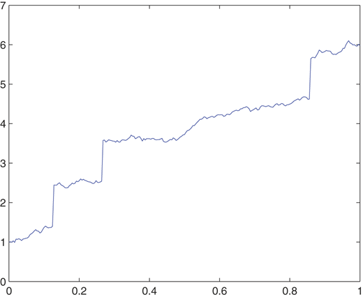
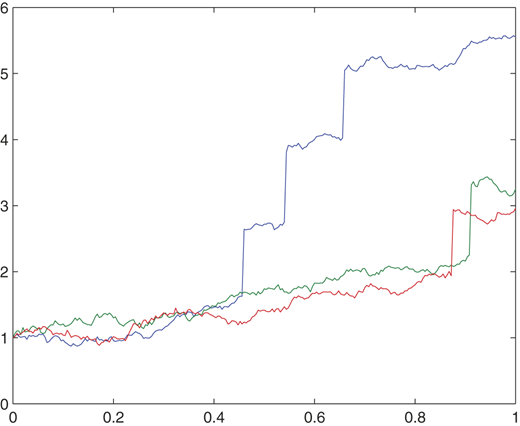
Recall that the optimal strategy $\hat{α} = {({\hat{τ}}_{n})}_{n \geq 0}$ is completely defined by the process Y and is obtained when Y reached successively the barriers L and U. As a result, solving numerically this strategy amounts to simulating sample path trajectories of the process Y. In recent years, several techniques have been proposed for the numerical solution of the process Y (for example the quantization algorithm, Malliavin calculus). Here the approximation by regression is chosen, which is well explained in [24, 25]. Our method is totally different from the method used in [26] which is based on the approximation of the Brownian and Poisson processes by a random walk. Recall once again that here the process X is the diffusion (4). For this application, a simple case of stochastic differential equation with jump is considered: Let $b, σ$ are constant drift and diffusion coefficients; $\tilde{μ} (d s, d e)$ gives an information about the jump: the probability of the jump happening at time t and the relative amplitude of the jump. It will be represented by a log-normal random variables, λ is the yearly average of the number of jumps. Thus the firm log-value is modeled as

X_{t} = x_{0} + b t + σ W_{t} + N_{t} - λ t .

By using the classical Euler scheme for sample path trajectories of the process X where $λ = 3, x_{0} = 1$ and $T = 1$ ⁠, one has: (see Figures 1 and 2).

Figure 1

View large Download slide

$b = 0.01, σ = 0.2$

Figure 2

View large Download slide

$b = 1, σ = 2$

Let us now focus on our problem: namely, how to simulate the process Y, and therefore the optimal strategy. Recall that

e^{- β t} g (t) = e^{- β t} (f (1, X_{t}) - f (2, X_{t})), L_{t} = - c_{1,2} e^{- β t}, U_{t} = c_{2,1} e^{- β t}, c_{1,2} and c_{2,1} > 0

which satisfy Hypotheses $(H_{1})$ and $(H_{2})$ ⁠.

First of all, when t tends to infinity, $Y_{t}$ goes to 0, so a finite horizon T should be fixed such that $t_{i} = i \frac{T}{n}, i = n, \dots, 0.$ More specifically, below the numerical samples show that as soon as $t \geq 1,$ the length of interval $(L_{t}, U_{t})$ is negligible.

$Y_{t} \in (L_{t}, U_{t})$ so the error is bounded by $U_{t} - L_{t}$ ⁠, the order of which being $e^{- β t} .$

To approximate the backward component $Y,$ the following discretization approximation scheme is introduced, for $0 = t_{0} < t_{1} < \dots < t_{n} = T$ ⁠:

{\begin{cases} {\tilde{Y}}_{T}^{π} = Y_{T}^{π} = 0 \\ {\tilde{Y}}_{t_{i}}^{π} = E_{t_{i}} [Y_{t_{i + 1}}^{π}] + (t_{i + 1} - t_{i}) e^{- β t_{i}} f (X_{t_{i}}^{π}) \\ Y_{t_{i}}^{π} = ({\tilde{Y}}_{t_{i}}^{π} \lor L_{t_{i}}) \land U_{t_{i}}, i \leq n - 1, \end{cases}

(56)

where $E_{t_{i}} = E [. | F_{t_{i}}] .$ To approximate the conditional expectation, here is adopted the Longstaff-Schwarz algorithm [25] which uses a regression technique (Least-Square Monte Carlo method). Taking the parameters $β = 0.5$ , $X_{0} = 1, b = 1, σ = 2,$ and the profits/costs functions

f (1, x) = 3 + 2 x^{-}, f (2, x) = 2 x^{+}, s o f (1, x) - f (2, x) = - 2 x + 3,

the evolution of Y is observed. Previously all the assumptions have to be checked:

(1)
One notes that with $X_{t} = b t + σ W_{t} + N_{t} - λ t,$ : Assumption $(H_{1}^{'})$ is satisfied since $f (i, x) = a + x^{\pm},$ so $E [{(a + X_{t}^{\pm})}^{2}] \leq 2 a^{2} + 2 E [(X_{t}^{2})] \leq 2 a^{2} + 6 (b^{2} t^{2} + σ^{2} t + λ t)$ thus $E [\int_{0}^{\infty} e^{- β t} f^{2} (i, X_{s}) d s] \leq \int_{0}^{\infty} e^{- β t} [2 a + 6 (b^{2} t^{2} + σ^{2} t + λ t)] d t < \infty .$

Interpretation: Recall once again that the optimal strategy $\hat{α} = {({\hat{τ}}_{n})}_{n \geq 0}$ is obtained when Y reached successively the barriers L and U. In Figures 3 and 4, the costs are higher than in Figures 5 and 6. In Figures 3 and 4, it could be not interesting to switch the technology. It is preferable that the firm takes the precaution of keeping long enough the technology 1, which will enable to obtain suitable expected profit.

Figure 3

View large Download slide

$L_{t} = - 0.5 e^{- 2 t}, U_{t} = 0.4 e^{- 2 t}$

Figure 4

View large Download slide

$L_{t} = - 0.5 e^{- 2 t}, U_{t} = 0.4 e^{- 2 t}$

Figure 5

View large Download slide

$L_{t} = - 0.02 e^{- 2 t}, U_{t} = 0.01 e^{- 0.2 t}$

Figure 6

View large Download slide

$L_{t} = - 0.02 e^{- 2 t}, U_{t} = 0.01 e^{- 2 t}$

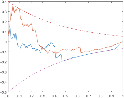
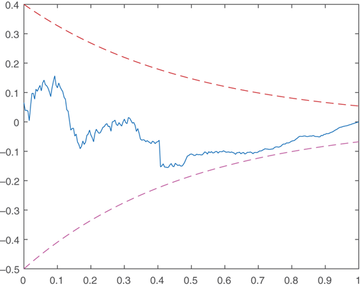
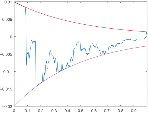
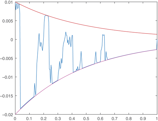
In the case of reasonable costs, as in Figures 5 and 6, the firm can switch the technology more often: actually at times $τ_{0} \sim 0.15$ and $τ_{1} \sim 0.97$ (Figure 5), respectively in Figure 5, the firm can switch the technology at times $τ_{0} \sim 0.05$ and $τ_{1} \sim 0.23$ ⁠.

The authors would like to thank Monique Jeanblanc for her constructive comments and suggestions to improve the quality of our work.

References

[1]

Hamadène

S

,

Jeanblanc

M

.

On the starting and stopping problem: application in reversible investments

.

Math Oper Res.

2007

;

32

(

1

):

182

-

92

.

Google Scholar

Crossref

[2]

Hamadène

S

,

Hassani

M

,

Ouknine

Y

.

Backward SDEs with two rcll reflecting barriers without Mokobodski's hypothesis

.

Bull Sci Math.

2010

;

134

:

874

-

99

.

Google Scholar

Crossref

[3]

Pardoux

E

,

Peng

SG

.

Adapted solution of a backward stochastic differential equation

.

Syst. Control Lett.

1990

;

14

:

55

-

61

.

Google Scholar

Crossref

[4]

Cvitanic

J

,

Karatzas

I

.

Backward stochastic differential equations with reflection and Dynkin games

.

Ann Probab.

1996

;

24-4

:

2024

-

56

.

Google Scholar

[5]

El Karoui

N

,

Pen

S

,

Quenez

MC

.

Backward stochastic differential equations in finance

.

Math Finance.

1997

;

7

(

1

):

1

-

71

.

Google Scholar

Crossref

[6]

El Karoui

N

,

Kapoudjian

C

,

Pardoux

E

,

Peng

S

,

Quenez

MC

.

Reflected solutions of backward SDE's and related obstacle problems for SDE's

.

Ann Probab.

Chicago: Institute of Mathematical Statistics

.

1997

;

25

(

2

):

702

-

37

.

Google Scholar

Crossref

[7]

Hamadène

S

,

Lepeltier

JP

,

Wu

Z

.

Infinite horizon reflected backward stochastic differential equations and applications in mixed control and game problems

.

Probab Math Stat.

1999

;

19

(

2

):

211

-

34

.

Google Scholar

[8]

Hamadène

S

,

Ouknine

Y

.

Reflected backward stochastic differential equation with jumps and random obstacle

,

Electron J Probab.

2003

;

8

(

2

):

1

-

20

.

Google Scholar

[9]

Hamadène

S

,

Hassani

M

.

BSDEs with two reflecting barriers driven by a Brownian and a Poisson noise and related Dynkin game

,

Electron J Probab.

2006

;

11

(

5

):

121

-

45

.

Google Scholar

[10]

Hamadène

S

,

Wang

H

.

BSDE's with two RCLL obstacles driven by Brownian motion and Poisson measure and a related mixed zero-sum game

.

Stoch Process Appl.

2009

;

119

(

9

):

2881

-

912

.

Google Scholar

Crossref

[11]

Pardoux

E

,

Peng

SG

. Backward stochastic differential equations and quasilinear parabolic partial differential equations. In:

Rozovskii

B.

and

Sowers

R.

(Eds).

Stochastic differential equations and their applications, Lect. Not. Cont. Inf. Sci.

Springer

.

1992

;

176

:

200

-

17

.

Google Scholar

Crossref

[12]

Hamadène

S

,

Ouknine

Y

.

Reflected backward SDEs with general jumps

.

Teor Veroyatnost i Primenen.

2015

;

60-22

:

357

-

76

.

Google Scholar

[13]

Chassagneux

JF

,

Elie

R

,

Kharroubi

I

.

Discrete time approximation of multidimensional BSDEs with oblique reflections

,

Ann Appl Probab.

2012

;

22

:

971

-

1007

.

Google Scholar

Crossref

[14]

El Asri

B

.

Optimal multi-modes switching problem in infinite horizon

.

Stochast Dynam.

2010

;

10-2

:

231

-

61

.

Google Scholar

[15]

Hu

Y

,

Tang

S

.

Multi-dimensional bsde with oblique reflection and optimal switching

.

Probab Theor Relat Field.

Springer Verlag.

2010

;

147

(

1-2

):

89

-

121

.

Google Scholar

Crossref

[16]

Akdim

K

,

Ouknine

Y

.

Infinite horizon reflected backward SDEs with jumps and right continuous left limited obstacle

.

Stochastic Anal Appl.

2006

;

24

:

1239

-

61

.

Google Scholar

Crossref

[17]

El Karoui

N

.

Les aspects probabilistes du Contrôle Stochastique

.

Lect Notes Math

.

Berlin

:

Springer-Verlag

;

1981

:

876

.

Google Scholar

Crossref

[18]

Amami

R

.

Application of doubly reflected BSDEs to an impulse control problem

.

Optim J Math Program Oper Res.

2013

;

62

(

11

):

1525

-

52

.

Google Scholar

[19]

Essaky

EH

.

Reflected backward stochastic differential equation with jumps and right continuous left limited obstacle

.

Bull Sci Math.

2008

;

132

:

690

-

710

.

Google Scholar

Crossref

[20]

Hamadène

S

,

Lepeltier

JP

,

Matoussi

A

.

Double barrier reflected backward SDE's with continuous coefficient

.

Pitman Res Notes Math Ser.

1997

;

364

:

161

-

75

.

Google Scholar

[21]

Dellacherie

C

,

Meyer

PA

.

Probabilités et Potentiel

.

Chap. I-IV

.

Paris

:

Hermann

;

1980

.

Google Scholar

[22]

Dellacherie

C

,

Meyer

PA

.

Probabilités et Potentiel

.

Chap. V-VIII

.

Paris:

Hermann

;

1982

.

Google Scholar

[23]

Jacod

J

,

Shiryaev

AN

.

Limit Theorems for Stochastic Processes

. (2nd ed.)

Springer-Verlag

;

2003

.

Google Scholar

Crossref

[24]

Huynh

HT

,

Lai

VS

,

Soumaré

I

.

Stochastic simulation and applications in finance with Matlab programs

.

John Wiley & Sons

;

2008

.

Google Scholar

Crossref

[25]

Longstaff

F

,

Schwartz

E

.

Valuing American options by simulation: a simple least-squares

.

Rev Financ Stud.

Spring, Oxford University.

2001

;

1-14

:

113

-

47

.

Google Scholar

[26]

Dumitrescu

R

,

Labart

C

.

Numerical approximation of doubly reflected BSDEs with jumps and RCLL obstacles

.

J Math Anal Appl.

Elsevier.

2016

;

442

(

1

):

206

-

43

.

Google Scholar

Crossref

Infinite horizon impulse control problem with jumps and continuous switching costs

1. Introduction

2. Preliminaries and problem formulation

3. The impulse control problem

4. Reflected BSDE with jumps and infinite horizon

4.1 Reflected BSDE in case of a single barrier, infinite horizon

4.2 Comparison theorem in case of a single barrier

4.3 Double barrier reflected BSDE with jumps and infinite horizon

4.3.1 Uniqueness of the solution

4.3.2 Existence of the solution for double barrier reflected BSDE with jumps

5. Application to the impulse control problem with infinite horizon

6. Numerical resolution

References

Further reading

Appendix

Email Alerts

Cited By

Infinite horizon impulse control problem with jumps and continuous switching costs Open Access

1. Introduction

2. Preliminaries and problem formulation

3. The impulse control problem

4. Reflected BSDE with jumps and infinite horizon

4.1 Reflected BSDE in case of a single barrier, infinite horizon

4.2 Comparison theorem in case of a single barrier

4.3 Double barrier reflected BSDE with jumps and infinite horizon

4.3.1 Uniqueness of the solution

4.3.2 Existence of the solution for double barrier reflected BSDE with jumps

5. Application to the impulse control problem with infinite horizon

6. Numerical resolution

References

Further reading

Appendix

Email Alerts

Suggested Reading

Related Chapters

Recommended for you

Cited By

Sharing Unavailable

Infinite horizon impulse control problem with jumps and continuous switching costs