


We segregate a region of interest into several zones, and consider the problem of estimating the zone of target sensor node using received signal power at the sensor node corresponding to the transmitted signal from each anchor node. Contrary to typical indirect zone estimation methods (location estimation followed by zone mapping), we propose direct zone estimation with maximum likelihood approach for Rayleigh and Nakagami-Rice fading channels. The advantage of the proposed approach is confirmed via computer simulations. However, the performance evaluation using measurement data has revealed the impact of non-uniform antenna beam patterns of practical sensor nodes. Thus, we also propose to incorporate the effect of the directivity of practical sensors in the evaluation of likelihood function, and demonstrate the validity of the proposed approach using measurement data.
1 Introduction
IoT (Internet of Things) sensors play a pivotal role in the realisation of smart cities, buildings, homes, offices, and factories. They are embedded in the infrastructure with wireless devices such as Bluetooth, Zigbee, and 802.15.4, and support monitoring and control of the surrounding environment. Typical monitoring and control applications include controlling air conditioners with embedded IoT temperature sensors in the office, controlling the brightness of lights with embedded IoT brightness sensors in the living room, notifying workers when they leave designated safety walkways on the factory premises using IoT sensors and so on. These IoT sensors could enable new applications by effectively leveraging existing infrastructure.
Most monitoring and control applications require the location information of people or devices in indoor environments. Depending on the required level of granularity of the location information, indoor positioning could be categorized into position estimation (fine-grained) and zone estimation (coarse-grained). Applications such as monitoring designated safety walkways require fine-grained location information. On the other hand, applications such as temperature or brightness control don’t require a fine-grained location information. Instead, a coarse-grained location should be estimated with high probability. Figure 1 shows an illustration of the use case scenario of zone estimation, where all the luminaires are Bluetooth enabled and the target sensor (smartphone carried by a person) could be in any location. Lights are turned on only in the person’s zone to reduce energy consumption.
Several methods for the fine-grained position estimation have been proposed that make use of sensor networks as in Shit et al.[16] and Niculescu and Nath [13]. Position estimation using IoT sensors could be categorized into two types, namely dedicated device approach and non-dedicated device approach. In the dedicated device approach, a dedicated distance measuring device embedded in IoT sensor is used to estimate the distance. And then, the position of target node is estimated using the distance information between target and anchor nodes (sensor nodes whose locations are known). For example, active bat [3] and cricket [14] use ultrasonic waves to measure the distance between nodes to estimate position. Dedicated device based methods can generally estimate the position with high accuracy, but have the disadvantage of high cost. In the non-dedicated device approach, wireless communication signals transmitted by IoT sensors are typically used for position estimation as in Yonezawa et al.[19] and Yick et al.[18]. For example, trilateration Manolakis [11], min-max Langendoen and Reijers [10], and Maximum Likelihood (ML) [8] use received signal power to estimate the position. Non-dedicated device based methods incur no additional cost, but the accuracy of estimated location is not as high as dedicated device based methods.
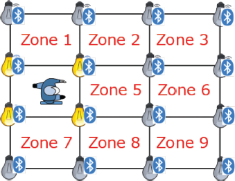
In coarse-grained zone estimation, a region of interest is divided into multiple zones, and a person or device could be in any one of these zones. The goal is to estimate the zone to which the person or device belongs. Zone estimation could be categorized into two types, namely indirect and direct approaches. Indirect zone estimation first estimates the target sensor position using one of the position estimation methods. The estimated position is then assigned to predetermined zones. In principle, any method of position estimation can be used for the indirect approach to zone estimation. On the other hand, direct approach estimates the target sensor zone without estimating the position. From a viewpoint of data-processing inequality [5], the direct zone estimation approach could be preferable to the indirect approach. To the best of our knowledge, schemes associated with the direct zone estimation have not been extensively studied, while the scheme based on naive received signal strength (RSS) is proposed in Warmerdam and Pandharipande [17]. This naive RSS scheme directly determines the target sensor zone by identifying the zone surrounded by anchors with the highest average RSS.
In this paper, we consider the problem of the direct zone estimation for IoT applications such as temperature or brightness control in indoor environments, and propose an ML based direct sensor zone estimation scheme using received signal power from anchor nodes observed at the target sensor node. We have presented preliminary results of the proposed approach based mainly on computer simulations in Honda et al.[9]. However, detailed analysis of the proposed approach using measurement data has revealed the large impact of the non-uniform antenna beam pattern of practical sensors on the zone estimation results, which was not considered in our preliminary study. Therefore, we have modified our algorithm by incorporating the directivity of the sensors into the likelihood function, where the directivity of practical sensors is obtained by pre-measurement. It should be noted here that we have numerically confirmed that not all, but only some samples of sensors are sufficient to pre-measure the directivity, which can greatly reduce the load of measurement and is beneficial from a practical deployment point of view. We have compared the performance of the proposed direct zone estimation method in terms of the zone detection rate with that of existing direct and indirect zone estimation methods with computer simulations and measurement data, and have demonstrated the validity of the proposed approach for the zone estimation problem.
The specific contributions of this journal version are listed below:
We have performed measurements in a wide area of around 110 square meters and evaluated zone detection rates of existing indirect zone estimation and proposed direct zone estimation with ML.
We have observed the impact of practical sensor’s non-uniform antenna beam patterns on zone detection rate, and have compensated this effect by incorporating directivity of practical sensors into likelihood function.
Since pre-measuring antenna beam pattern of each sensor is a tedious task, we have considered the possibility of re-using a sample sensor device’s beam pattern to other sensor devices of the same type.
We have compared the zone estimation performance of the proposed direct ML approach with the naive RSS scheme proposed by Warmerdam and Pandharipande [17], as well as indirect zone estimation approach using competitive position estimation schemes including the ML based method [8], the trilateration method [11] and the min-max method [10].
The rest of the paper is organized as follows. Section 2 explains the direct zone estimation problem and received signal model. Section 3 explains the proposed direct zone estimation method with ML. Section 4 explains the simulation scenario along with evaluation results. Section 5 explains the measurement scenario along with evaluation results, followed by concluding remarks in Section 6.
2 Direct Zone Estimation Problem and Received Signal Model
2.1 Problem Definition
The assumptions on the problem setting are as follows:
Q anchor nodes (c1, c2, ⋯,cQ) are placed at pre-determined known locations.
- A target sensor node u, whose position is unknown, is placed in the area where the anchor nodes are located.Figure 2
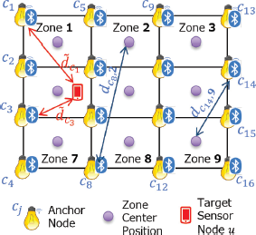
Example of node placement for Q = 16.
Each anchor node cj transmits radio signals N times, where L symbols are included in each transmission.
Under these assumptions, we consider the problem of estimating the zone to which the target sensor node u belongs using the received signal power at the sensor node u corresponding to the transmissions from Q anchor nodes. Figure 2 shows an example of the arrangement of anchor nodes when they are placed on regular grids with Q = 16. Here, in the case of Figure 2, each zone is defined as a minimum region surrounded by four anchor nodes, where the zone is denoted by w ∈ {1, 2, ∈, R} and R is the number of zones. Let denote the distance between the anchor node cj and the sensor node u, and denote the distance between the anchor node cj and the center of zone w. The zone to which the sensor node u belongs is represented as wu. Thus, the problem of zone estimation results in the estimation of the zone index wu.
In the following sections, we describe received signal model at the sensor node u for two different channel models, namely, Rayleigh fading channel model and Nakagami-Rice fading channel model.
2.2 Received Signal Model
2.2.1 Received Signal Model in Rayleigh Fading Channel
In this section, we assume that channels between nodes are modeled as frequency non-selective Rayleigh fading channels with path loss. The received signal at the sensor node u for the lth transmitted symbol in the nth transmission period from the anchor node cj can be written as
where is the lth transmitted symbol in the nth transmission period from the anchor node cj with mean 0 and is the channel coefficient between anchor node cj and the sensor node u in the nth transmission period from the anchor node cj including the impact of transmit power and antenna beam pattern, is the complex white Gaussian measurement noise with mean 0 and variance , and ℂ is the set of all complex numbers. The channel coefficient follows a complex Gaussian distribution with mean 0 and variance which is given by
where α is the path loss exponent, P is the transmit power from each anchor node, is the antenna directivity gain of anchor node cj in the direction of sensor node u, and is the directivity gain of sensor node u in the direction of cj. We assume block fading channels, where the channel coefficients are constant during one transmission period of L symbols, but vary independently in different transmission periods. In order to take the path loss into consideration, we have measured the average received power when a signal is sent with transmit power of P as 1 and with inter-node distance of dref, and use this value as a reference. Note that the impact of antenna directivity gains is considered while measuring the reference average received power.
Defining the received signal vector at the sensor node u composed by L received symbols in the nth transmission period from the anchor node cj as
the instantaneous total received power at the sensor node u in the nth transmission period from the anchor node cj is given by
Here, since and are assumed to be uncorrelated, we approximate as
and
Then, can be approximated as
2.2.2 Received Signal Model in Nakagami-Rice Fading Channel
Next, we consider the case where channels between nodes are modeled as frequency non-selective Nakagami-Rice fading channels with path loss. The received signal at the sensor node u for the lth transmitted symbol in the nth transmission period from the anchor node cj is given by
where is the channel coefficient between anchor node cj and the sensor node u in the nth transmission period from the anchor node cj including the impact of transmit power and antenna gains, and it follows a complex Gaussian distribution with mean and variance
Here, is the amplitude corresponding to the line-of-sight (LoS) path between the sensor node u and the anchor node represents the measured average received power of the scattered wave component when a signal is sent with transmit power of P = 1 and with inter-node distance dref and pre-measured antenna directivity gains. The Rician factor K is the ratio of the power of the LoS component to that of the scattered component and is expressed as
The instantaneous total received power at the sensor node u in the nth transmission period from the anchor node cj is given by
3 Proposed Direct Zone Estimation with Maximum Likelihood
ML estimation is an approach to estimate parameters in the probability distribution from the observed samples using likelihood function. In the zone estimation problem considered in this paper, the instantaneous total received power is used as the sample, and the unknown parameter to be estimated is the index wu of the zone to which the sensor node u belongs.
3.1 Maximum Likelihood Direct Zone Estimation in Rayleigh Fading Channel Model
In order to simplify the problem, we first approximate the position of target sensor node u to be at the center of the zone wu for sensor zone estimation. Then, the channel coefficient in (7) follows a complex Gaussian distribution with mean 0 and variance
Note that wu is the zone index. Thus, indicates the gain of the anchor node cj in the direction of the center of zone wu, and indicates the gain of the sensor node assuming it is located at the center of zone wu to the anchor node cj. In order to derive the conditional probability density function (PDF) of in (7) given the zone index wu to which the sensor node u belongs, we define
and rewrite as
Since the sum of squares of two independent Gaussian random variables follows an exponential distribution [15], the conditional PDF of given wu is written as
On the other hand, since the sum of independent exponential random variables follows the Erlang distribution [6], the PDF of is given by
Moreover, since the PDF of the sum of independent random variables is a convolution of each PDF [7], the conditional PDF of given wu is written as
where Γ(x) and Γ(a, x) represent the gamma function and the incomplete gamma function, respectively, which are defined as
From (18), assuming that the instantaneous total received powers at the sensor node u from different anchor nodes are independent, the likelihood function when the instantaneous total received power from all anchor nodes is observed at the sensor node u is given by
Moreover, assuming that the instantaneous received power at each transmission period is independent, the ML estimate of the zone index to which the sensor node u belongs is obtained by solving the optimization problem of
with exhausitive search.
3.2 Maximum Likelihood Direct Zone Estimation in Nakagami-Rice Fading Channel Model
Approximating the position of sensor node u to be center of the zone wu, the channel coefficient in (11) follows a complex Gaussian distribution with mean and variance
where denotes the amplitude corresponding to the LoS path between the center of the zone wu and the anchor node cj, and the Rician factor K can be written as
Defining
in (11), can be written as
The conditional PDF of given wu is written as (for detailed derivation, see Appendix)
where I0 (z) denotes the zero-order modified Bessel function of the first kind defined as
Since the PDF of is given by (17), the conditional PDF of given wu can be obtained by the convolution of and , but it is difficult to obtain it in a closed form because contains the zero-order modified Bessel function of the first kind. The zero-order modified Bessel function of the first kind can be approximated by the exponential function when the Rician factor K is large, but it is still difficult to calculate the convolution even with this approximation. Therefore, we use the property that the Nakagami-Rice distribution can be approximated by the Nakagami-m distribution NAKAGAMI [12]. The PDF of the Nakagami-m distribution is expressed as
Using the Nakagami-m distribution, the conditional PDF of given wu is written as
where and are given by
respectively. Thus, the conditional PDF of given wu is obtained as
by the convolution of (17) and (31), where 1F1(a; b; z) denotes the general hypergeometric function defined as
From (34), assuming that the instantaneous total received powers at the sensor node u from different anchor nodes are independent, the likelihood function when the instantaneous total received power from all anchor nodes is observed at the sensor node u is given by
Thus, the ML estimate of the zone index to which the sensor node u belongs is obtained by solving the optimization problem of
with exhaustive search assuming that the instantaneous received power at each transmission period is independent.
4 Simulation Results
In this section, we compare the estimation success probabilities of the proposed ML-based direct zone estimation with naive RSS scheme-based direct zone estimation [17], as well as indirect zone estimation methods using existing position estimation methods, such as the existing ML [8], the trilateration [11], and the min-max [10], by computer simulations to demonstrate the validity of the proposed approach. Note that, in all simulations in this section, we assume ideal omni-directional antenna both for the transmission from anchor nodes and for the reception at the sensor node for simplicity, and also because it is not straightforward to take non-uniform antenna beam pattern into consideration in the indirect zone estimation approach.
4.1 Simulation Specifications
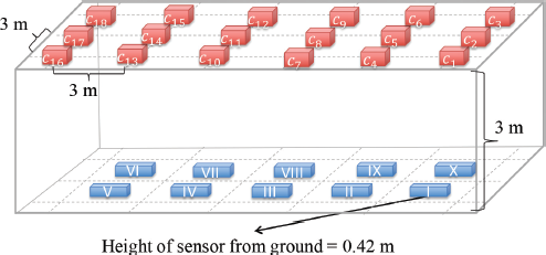
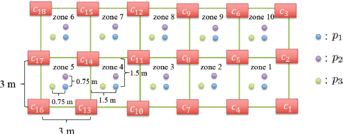
Figure 3 shows the arrangement of the nodes used in the simulations. The anchor nodes are placed on 3 × 6 regular grid points on the ceiling of the three-dimensional space. The grid spacing is set to 3 [m], and the height from the ground to the ceiling is set to 3 [m]. Ten sensor nodes (I to X) are placed at a height of 0.42 [m] from the ground. Figure 4 shows a view of the node arrangements shown in Figure 3 from above, where each zone is defined as a minimum region surrounded by four anchor nodes. We consider three possible scenarios for each sensor node: center of the zone (p1, blue), 0.75 [m] upward from the center (p2, purple), and 0.75 [m] to the left (p3, green), as shown in Figure 4. We evaluate the performance in two different channel models, namely, Rayleigh fading channel model and Nakagami-Rice fading channel model. The zone to which the sensor node belongs is estimated from the received signal power at the sensor node for transmission from all anchor nodes. This trial is repeated 100 times and the performance is evaluated using the average estimation success rate of the 10 locations. The path loss exponent is set to α = 2.35. The transmit power is set so that the average signal-to-noise power ratio (SNR) when the signal is received by a node at a distance of dref = 3.34 m from the transmission node is 10 [dB]. For Nakagami-Rice fading channel model, the Rician factor is set to K = 10. We perform the zone estimation using K and α as parameters, and take the value when the success rate of the zone estimation is the highest as the estimated value of these parameters.
4.2 Simulation Results in Rayleigh Fading Channel Model
Figures 5–10 show the simulation results of the estimation success rates of the proposed direct zone estimation with ML approach, naive RSS approach, indirect zone estimation using position estimation methods namely the minmax method, the trilateration, and the existing ML, assuming that the received SNR = 10 [dB], the number of transmitted symbols L =1, 3, and the channel between nodes is assumed to be Rayleigh fading channel, when sensor nodes are placed at p1, p2, and p3, respectively. From Figures 5–10, we can see that the direct zone estimation methods outperform indirect zone estimation methods. Specifically, the proposed direct ML approach has the highest estimation success rates than the other methods for all cases. In the proposed direct ML approach, the estimation success rate increases with the increase in the number of symbols L transmitted at a time for the same number of transmissions. This is because the effect of measurement noise can be suppressed by increasing the number of transmitted symbols in each transmission. In addition, the estimation success rate increases as the number of transmissions increases, and for the case with L = 3 and the sensor location p1, the estimation success rate reaches 100% when the number of transmissions is 8 or more. This is because both the effects of fading and the measurement noise can be suppressed by multiple transmissions. We can also see that the estimation success rate decreases when the sensor nodes are placed at off center positions (i.e., p2 or p3). This is because the node locations are approximated to the center of the zone in the likelihood function of the proposed method. Nevertheless, for the case where L = 3 and the sensor nodes are placed at p2 or p3, the estimation success rate reaches 98% or more when the number of transmissions are 10.
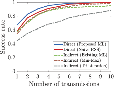
Estimation success rate versus number of transmissions (Rayleigh fading, sensor node placed at p1, number of transmitted symbols L = 1).
Estimation success rate versus number of transmissions (Rayleigh fading, sensor node placed at p1, number of transmitted symbols L = 1).
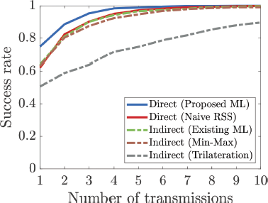
Estimation success rate versus number of transmissions (Rayleigh fading, sensor node placed at p1, number of transmitted symbols L = 3).
Estimation success rate versus number of transmissions (Rayleigh fading, sensor node placed at p1, number of transmitted symbols L = 3).
4.3 Simulation Results in Nakagami-Rice Fading Channel Model
Figures 11–12 show the simulation results of the estimation success rates of the proposed direct ML approach, naive RSS approach, and indirect zone estimation methods using the min-max method, the trilateration, and the existing ML approaches in the Nakagami-Rice fading channel model with the sensor location of p1 assuming that the received SNR = 10 [dB]. From Figures 11–12, we can see that the estimation success rate of the proposed method is the highest among all methods and the estimation success rate of the proposed method improves when the number of symbols L transmitted increases for the same number of transmissions. In addition, compared to the case of Rayleigh fading channel model (Figure 5), the estimation success rate is higher in the case of Nakagami-Rice fading. This is because in the Nakagami-Rice fading channel model, the received power variation is small due to the existence of the LoS path.
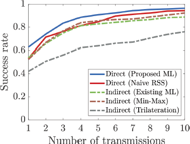
Estimation success rate versus number of transmissions (Rayleigh fading, sensor node placed at p2, number of transmitted symbols L = 1).
Estimation success rate versus number of transmissions (Rayleigh fading, sensor node placed at p2, number of transmitted symbols L = 1).
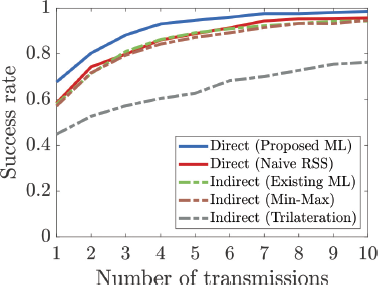
Estimation success rate versus number of transmissions (Rayleigh fading, sensor node placed at p2, number of transmitted symbols L = 3).
Estimation success rate versus number of transmissions (Rayleigh fading, sensor node placed at p2, number of transmitted symbols L = 3).
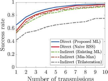
Estimation success rate versus number of transmissions (Rayleigh fading, sensor node placed at p3, number of transmitted symbols L = 1).
Estimation success rate versus number of transmissions (Rayleigh fading, sensor node placed at p3, number of transmitted symbols L = 1).
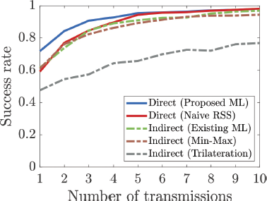
Estimation success rate versus number of transmissions (Rayleigh fading, sensor node placed at p3, number of transmitted symbols L = 3).
Estimation success rate versus number of transmissions (Rayleigh fading, sensor node placed at p3, number of transmitted symbols L = 3).
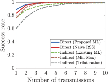
Estimation success rate versus number of transmissions (Nakagami-Rice fading SNR = 10 [dB], number of transmitted symbols L = 1).
Estimation success rate versus number of transmissions (Nakagami-Rice fading SNR = 10 [dB], number of transmitted symbols L = 1).
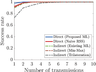
Estimation success rate versus number of transmissions (Nakagami-Rice fading SNR = 10 [dB], number of transmitted symbols L = 3).
Estimation success rate versus number of transmissions (Nakagami-Rice fading SNR = 10 [dB], number of transmitted symbols L = 3).
5 Measurement Results
In the previous section, we have assumed ideal omni-directional antennas at all nodes in order to clarify the basic performance of the proposed approach. In actual environments, however, common devices have non-uniform beam patterns, which would have some impact on the zone estimation. In this section, taking non-uniform beam patterns of devices into consideration, we compare the estimation success rates of the proposed direct ML method with naive RSS scheme by using measurement data. Note that, in this section, we evaluate the performance of direct zone estimation schemes only, because it is not straightforward to incorporate non-uniform beam patterns into indirect zone estimation approach.
5.1 Experiment Specifications
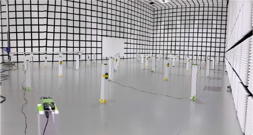
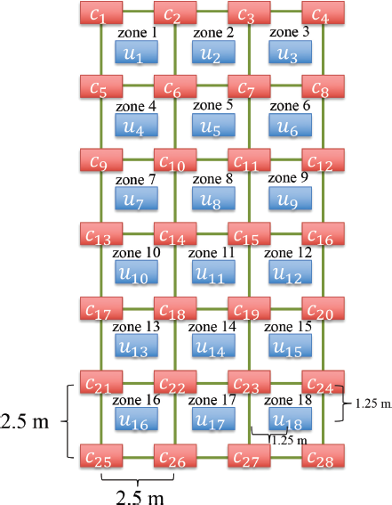
The performance of the proposed ML approach is evaluated with an experimental setup as shown in Figure 13. The experiment is performed in anechoic chamber with radio wave absorbers on five sides except the ground. The arrangement of nodes is shown in Figure 14. The anchor locations are on 4 × 7 regular grid points with 2.5 [m] spacing (shown in Figure 14 as c1 to c28), resulting in 18 zones in the area of interest. The sensor to be located is placed at the center of each zone (shown in Figure 14 as u1 to u18).
Nordic’s nRF52840 modules [1] are used as the nodes placed at the anchor locations and the sensor locations. As the standard BLE (Bluetooth Low Energy) [2] uses 40 channels spaced 2 [MHz] apart, the received signal power is measured between the node at each anchor location and the sensor location in 40 BLE channels. To achieve this in a time efficient way, a multi-channel TDMA protocol named “multi-spin” (as detailed in Bocca et al.[4]) is used. Multi-spin defines the order of transmission of sensors and synchronizes their switching on different frequency channels [4]. Multi-spin protocol is implemented on Nordic’s module with 40 BLE channels and accumulated received signal power among sensors. The received power measured at different BLE channels can be regarded as the received power at different transmission periods in the received signal model of Section 2. Therefore, we can reasonably assume that the number of BLE channels corresponds to the number of transmissions. We measure the instantaneous received power at the sensor location, and zone estimation is performed using the instantaneous received power of 40 BLE channels, where the received power for every combination of the anchor location and the sensor location is available.
5.2 Pre-Measurement of Antenna Beam Pattern
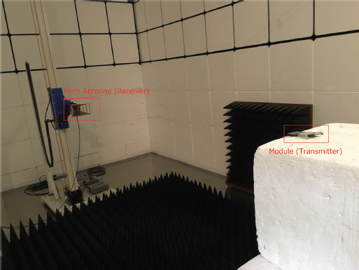
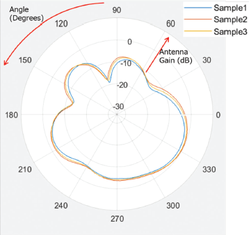
As the beam pattern is not omnidirectional in practical sensors or modules, beam pattern of three sample modules are measured in an anechoic chamber with radio wave absorbers on five sides except the ground as shown in Figure 15. Target module is kept on a rotating device with a resolution of 1 degree. Signal strength of transmitted beacon from the module is measured by the horn antenna whose radiation pattern is known in advance. Measured beam patterns of three sample modules are shown in Figure 16. Average antenna gains of three sample modules are -6 dB, -5 dB, and -5 dB, respectively. Although the beam patterns are similar, there are slight deviations in the average gains.
5.3 Measurement-Based Evaluation of the Estimation Success Rates
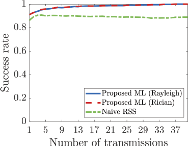
Figure 17 shows the estimation success rate performance of the proposed direct ML approach and the naive RSS scheme with the sensor location at the center of each zone using beam pattern of Sample 1 in Figure 16 for all nodes in common. In the proposed method, we have assumed Rayleigh or Nakagami-Rice fading channel models. From the figure, we can see that the proposed direct ML approach can achieve better performance than the naive RSS scheme for the case with actual measurement data as well.
Table 1 shows the estimation success rates of the proposed direct ML approach assuming Rayleigh or Nakagami-Rice fading channel models with the sensor location at the center of each zone and the number of transmissions as 40. We have evaluated the performance of the proposed methods for 4 different cases regarding the antenna beam pattern, namely, without considering beam pattern, using beam pattern of Sample 1 in Figure 16 in common for all nodes in the evaluation of the likelihood function, using beam pattern of Sample 2, and using beam pattern of Sample 3. From the table, we can see that higher success rate is achieved by considering antenna beam pattern, which demonstrates the large impact of antenna beam pattern on the estimation performance. Moreover, we can also see that the estimation success rate is almost the same regardless of the choice of sample beam pattern. This may imply that we can use a measurement beam pattern of a certain sensor device to calibrate all sensor nodes, which greatly reduces the effort required for measuring beam patterns. In addition, the proposed scheme with Nakagami-Rice model with the K factor of 0.4 achieves better performance than the proposed method with Rayleigh model, while the difference is rather marginal. Despite the presence of a LoS path between the transmitter and receiver in the measurements in the anechoic chamber, it seems that reflections and scattering from the ground and other devices (such as sensor modules, battery packs, and cables) have created the multipath fading environment.
6 Conclusion
In this paper, we have proposed a direct method to estimate a zone of the target sensor node from the information of the received signal power at target sensor node corresponding to transmitted signals from multiple anchor nodes using the ML approach.
From the computer simulation results of the zone estimation success rate, it is evident that the proposed direct zone estimation method outperforms existing direct zone estimation scheme and indirect zone estimation schemes using existing position estimation methods in the case of both Rayleigh and Nakagami-Rice fading channel models. The outcome remains unchanged even if the zone position is slightly shifted away from the center of zone.
From the zone estimation performance evaluation using measurement data, it is observed that the non-uniform beam patterns of practical sensor devices have large impact on the zone estimation performance. Therefore, we compensated this effect by incorporating the antenna directivity of sensor device into likelihood function. From the numerical results of the zone estimation rate using the measurement data, it is clear that the proposed direct zone estimated method with ML could be used in practical scenarios.
Future works include the performance evaluation of the proposed method in a real-time scenario and the assessment of the impact of the way of holding wireless devices by mobile users on the beam pattern.
Appendix
Probability Density Function (PDF) of Magnitude Square of Complex Gaussian Random Variable with Non-zero Mean
Consider a complex Gaussian random variable U = X + iY with mean a(∈ ℂ) = are + iaim and variance σ2, where X and Y are the real part and the imaginary part of U. Target is to deduce the PDF of Z = |U|2.
As X and Y are real Gaussian random variables following N(are, σ2/2) and N(aim, σ2/2) respectively, PDFs of X and Y are represented as
and
The joint PDF of X and Y is given by
With the variable transformation to the polar coordinates by setting x = r cos θ and y = r sin θ in the above equation, the joint PDF pR,Θ(r, θ) is given by
where β satisfies
Next, the PDF of R is deduced from (41) by the marginalization with respect to
Thus, the pdf of Z = |U|2 is finally given by

