


Single-channel speech enhancement aims to remove the interfering noise and reverberation in real environments by a single microphone, which is a very challenging task in the speech signal processing field. Over the past years, deep learning has shown great potential for speech enhancement. In this paper, we propose a novel real-time framework, called DBCN, which is a dual-branch architecture. One branch takes waveform as its input for time-domain modeling and the other one takes shift real spectrum as input for frequency-domain modeling. The two branches have the same network structure, which is the representative convolutional recurrent network. To exchange information sufficiently, a bridge module is added between the two branches. Furthermore, we propose a novel feature normalization approach that enables each band to complete the normalization independently by counting the root mean square of each band and obtaining the inter-frame relationship for each band. The proposed approach allows the network to ignore the magnitude during processing, reducing learning difficulty and improving performance. Systematical evaluation and comparison are conducted. Experimental results show that the proposed system substantially outperforms related algorithms for causal and non-causal speech enhancement under very challenging environments.
1 Introduction
Teleconferencing is becoming more and more popular at present, particularly during the COVID-19 pandemic. However, various noises in real environments can severely interfere with normal speech communication. To recover clean speech from the noise-contaminated mixture, speech enhancement is indispensable in almost all speech communication devices. Although the study of speech enhancement has a long history and many methods are invented in the literature [20], it is still a challenging task in practice, particularly for the single-channel scenario where only one microphone is available.
Spectral subtraction [2] is a classic method for single-channel speech enhancement, which subtracts the estimated spectrum of noises from the mixture. However, it is very difficult to estimate the spectrum of non-stationary noise which varies dramatically with time, and spectral subtraction becomes invalid in this most common scene. To overcome the shortcomings of traditional speech enhancement methods [2, 5, 37], Wang et al. first introduced a deep neural network for speech separation [48], which decomposes the input mixture into time-frequency representation and estimate the time-frequency (T-F) binary mask to recover the clean speech. The experimental results showed the great potential of DNN for speech enhancement task.
Since then, a large number of methods for speech enhancement using deep learning have been extensively studied, most of which exploit the T-F structure. Their training objectives can be divided into two main streams, one is masking-based and the other is mapping-based. For the masking-based targets, such as ideal binary mask (IBM) [44] and ideal ratio mask (IRM) [47], the network models the relationship between noisy speech and clean speech, and the mask is learned to cover the noisy speech to remove noise. For the mapping-based targets [21], such as spectral magnitude and complex spectral, the network learns a mapping and directly outputs clean speech. The training target together with the input features trains a DNN and obtains the enhanced waveform by reconstructing the estimated target.
Since phase is difficult to estimate, the early enhancement methods [18, 40] only enhance the magnitude and use the noisy phase for reconstruction. One example is the convolutional recurrent network (CRN) proposed by Tan et al. [40], which incorporated convolutional encoder-decoder (CED) and long short-term memory (LSTM) into the CRN architecture, and finally trained a magnitude-based mapping network. However, subsequent research has shown that incorporating phase into the supervised learning step can be effective in enhancing the listener’s subjective perception [27]. At present, many approaches combining magnitude enhancement and phase perception have been proposed [13, 46, 52, 54, 55], which can be roughly classified into time-domain speech enhancement and complex frequency-domain speech enhancement. In complex spectrogram enhancement, the real and imaginary components of the complex-valued noise STFT (Short Time Fourier Transform) are simultaneously enhanced to recover the complex spectrogram of clean speech, and also indirectly recover the phase information by learning the relationship of the RI component information [11, 15, 16, 25, 41, 50]. Compared with complex frequency-domain approaches, time-domain methods [10, 17, 22, 26, 29, 30, 34] have several obvious advantages. First, STFT for frequency domain processing usually requires multiple vibration periods in one frame to analyze the frequency characteristics, while time domain processing has no requirement for frame length. This means that temporal networks can model data at a finer scale. Second, the time-domain approach avoids the computations associated with converting between the two domains. That is, the raw speech is used directly for regenerated speech enhancement without going through the STFT process. Luo et al. used time-domain models for speech separation, and successively proposed TasNet, Conv-TasNet and DPRNN [22-24]. All of them used extremely small frame lengths to replace the STFT, which greatly improved the performance of the model. Subsequently, many similar methods have been widely explored in the field of speech enhancement [7, 31, 33, 51]. However, time-domain methods usually require more trainable parameters and greater model complexity, which is difficult to apply in practical scenarios. Therefore, making full use of their respective advantages is still a problem worth exploring.
Most mainstream enhancement models are still trained either in frequency or in time domain, and some researchers use cross-domain constraints or cross-domain training for speech enhancement. Pandey et al. [30] combined the loss of the time-domain waveform and the loss of the frequency domain in a certain ratio to train the model, and Wang et al. [45] stringed together three different domain modules for cross-domain joint training. Both of them achieve great performance. In fact, the superiority of the cross-domain model is theoretically based. Models in different domains may play different roles in dealing with different types of noise. For impulse noise as shown in the left column of Figure 1, it is easy to eliminate in the time domain. Only a few samples need to be removed. When it comes to the frequency domain, the noise pollutes the entire frequency band, and it is difficult to be eliminated on the frequency domain. In contrast, for a narrow band noise like a pure tone as shown in the right column of Figure 1, the noise is distributed on the narrow band and the frequency domain-based method covers well. In the time domain, the noise and the speech are coupled together at every sample, and it is hard to decouple on time domain. Therefore, we proposed a dual-branch network architecture [53] processing on both frequency- and time-domain, and the experimental results show impressive enhancement performance.
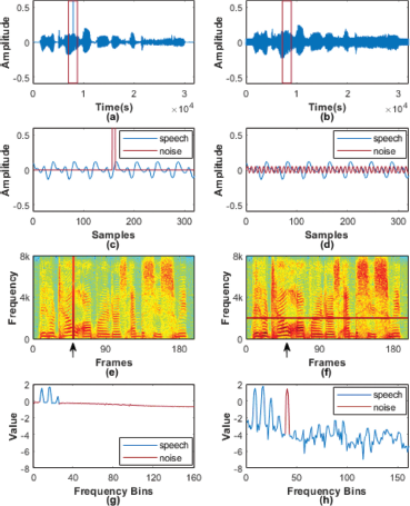
Here is a schematic diagram illustrating the difference between impulse noise and narrow-band noise. The left column contains: (a) the waveform of a mixed speech with impulse noise, (c) the waveform diagram of the frame inside the red box in (a), (e) the log power spectrum corresponding to the waveform in (a), (f) the frequency diagram of the frame which is pointed out in (e) by an arrow. The right column contains corresponding schematic representations of mixed speech with narrow-band noise.
Here is a schematic diagram illustrating the difference between impulse noise and narrow-band noise. The left column contains: (a) the waveform of a mixed speech with impulse noise, (c) the waveform diagram of the frame inside the red box in (a), (e) the log power spectrum corresponding to the waveform in (a), (f) the frequency diagram of the frame which is pointed out in (e) by an arrow. The right column contains corresponding schematic representations of mixed speech with narrow-band noise.
The dual-branch network consists of two convolutional recurrent networks (CRN) to process the time and the frequency representations respectively. At the same time, two branches exchange information after each convolution except the output layer. The key idea is to learn feature representations from two different perspectives in the time domain and the frequency domain and provide the learned features for each other as a reference to improve performance. From the complementary perspective, the time domain branch directly enhances the original speech, which avoids the problem of signal distortion caused by invalid STFT [8]. In addition, the time domain calculates all the discrete sample points, resulting in more attention to detail and prompting the network to eliminate some time-sensitive noises. In contrast, the frequency domain branch is responsible for suppressing the main noise components and eliminating frequency-sensitive noise. Note that we convert the complex spectrum to shift real spectrum (SRS) [38] losslessly to ensure that all operations of the network are in the real-valued domain and make the interaction of the two branches smooth. The contributions of this work are as follows,
We propose a dual-branch convolutional network structure that combines time-domain and frequency-domain processing. We use a bridge layer to facilitate the flow and fusion of cross-domain information. This allows our model to effectively exploit the complementary nature of these two domains and improve performance. By fully comparing our approach with multiple baseline methods, we demonstrate the effectiveness of our proposed network structure.
Based on the dual-branch convolutional network, we propose a novel feature normalization method. This method normalizes each frequency band independently by calculating the root mean square of each frequency band. It makes the network independent of the input amplitude and leads to better generalization ability for real-time scenarios.
We conducted a preliminary exploration of the information fusion layer and investigated the effects of different initialization methods on the performance of the fusion layer. This research forms the basis for further development and optimization of the fusion layer in our proposed network structure.
We used three different combinations of loss functions to constrain the time-domain branch and the frequency-domain branch separately. This allowed us to investigate the behavior of our network under different loss function configurations and validated the superiority of the proposed cross-domain loss function combination. We also conduct ablation experiments to evaluate the contribution of the proposed modules.
The remainder of the paper is organized as follows. In Section 2, the time-domain speech enhancement problem and shift real spectrum transformation are described. In Section 3, we present the proposed dual-branch network in detail. In Section 4, the experimental setting and data setup are given. Experimental results are displayed along with the analysis in Section 5. Finally in Section 6 we conclude the paper.
2 Problem Formulation
2.1 Monaural Speech Enhancement
Given a single-microphone noisy mixture m, monaural speech enhancement aims to separate target speech s from background noise n. A noisy mixture can be formulated as:
where k denotes the time index.
In the time domain, the algorithm aims to get s directly from mixture y rather than a T-F representation of y. The process for time-domain speech enhancement using DNN can be expressed as:
where ϕθ represents a function defined by a DNN model parameterized by θ. Generally, a speech enhancement network is designed to process frames of the speech signal. Given a speech signal s, it is first chunked into overlapping frames before being processed by the DNN model ϕθ. Let M denote a matrix consisting of frames of the signal m, and Mt denote the tth frame of the signal, then Mt can be formulated as:
where K is the frame length and J is the frame shift. The number of frames T is calculated from the signal length L and the frame shift J and expressed as , where ⌊⌋ denotes the floor function. Then a target frame can be computed by:
where ŝt is computed using Mt, T1 past frames, and T2 future frames.
2.2 Shift Real Spectrum (SRS)
In addition to the time domain, noisy speech is usually processed in the T-F domain. The two major frequency-domain methods are to enhance speech on the magnitude spectrum and the complex spectrum, respectively. The former ignores the phase and couples the predicted magnitude with the noisy phase in the recovery phase, causing a deviation from the target speech. The latter models the real and imaginary parts at the same time, which requires further exploration of the relationship between the real and imaginary parts and also brings large complexity. Soni et al. proposed an alternative to complex spectrum in their study [38], called shift real spectrum (SRS). By applying SRS, frequency domain information can be learned in the real field [19].
Given a time-domain speech s, we can use discrete-time Fourier transform (DTFT) to obtain a complex spectrum S which consists of a real part (denoted as SR) and an imaginary part (denoted as SI). As such, S = SR + jSI where j is an imaginary unit, and the speech s can be expressed as (SR, SI) losslessly. More specifically, the real part SR is an even function that consists of a series of cosine basic functions, while the imaginary part SI is an odd function that stands for a superposition of a series of sine functions. That is, any signal s in the time domain can be described as:
where seven and sodd denote the IDTFT(SR) and IDTFT(j • SI), respectively. When the signal s is an odd function, the even part can be ignored because sodd = 0. Likewise, the odd part can be ignored when the signal is an even function. By padding the signal with zeros of appropriate length as Figure 2 shown, we can decompose the signal into an even and an odd function, whose amplitude is half of the signal s. Thus, the original signal can be described as s = 2 • I DT FT (SR). In practice, we first separate the signal into windowed frames. Then we apply STFT to these windowed frames. Finally, the real part is taken as the representation. In the remainder of this article, all the mentioned STFT processes are performed in this way.
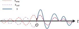
An example of zero-padded singal. The blue line is the original signal. The red and purple dashed lines denote the odd and even signals, respectively.
An example of zero-padded singal. The blue line is the original signal. The red and purple dashed lines denote the odd and even signals, respectively.
3 Dual-Branch Architecture
In this section, the details of the proposed dual-branch network are introduced. As shown in Figure 3, the proposed dual-branch network consists of two main modules: the time-domain module CRN-Time and the frequency-domain module CRN-SRS. The input of the two-branch network is a noisy mixture. CRN-Time module takes 320-point frames with 160-point overlapping as input and generates a time-domain estimate of the clean frames which is then converted back to speech. The CRN-SRS module takes the SRS obtained by the ISRS operation as input and estimates the clean SRS representation. Note that each branch has an independent output and the output of CRN-SRS is obtained by ISRS. We adopt the same structure for the time domain branch and the frequency domain branch. This makes the features of the two branches have the same dimension, which ensures the smooth flow of information in the two domains. Secondly, since the best feature conversion structure has not been found for the time being, we hope to achieve the SRS-liked transformation by using the trainable parameters, which also require the same dimension. In the following subsections, we will introduce several key modules, network configurations, and loss functions.
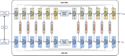
A schematic diagram illustrating the dual-branch architecture. The upper module CRN-Time employs a CRN to predict the temporal representation, the lower module CRN-SRS employs the same structure to predict the frequency-domain representation. After each layer of convolution, a bridge layer is used for feature conversion and fusion. Each module get an output and the output of CRN-SRS represents the outcome of the proposed network because of its better performance in the evaluation stage.
A schematic diagram illustrating the dual-branch architecture. The upper module CRN-Time employs a CRN to predict the temporal representation, the lower module CRN-SRS employs the same structure to predict the frequency-domain representation. After each layer of convolution, a bridge layer is used for feature conversion and fusion. Each module get an output and the output of CRN-SRS represents the outcome of the proposed network because of its better performance in the evaluation stage.
3.1 Gated Convolution And Grouping Strategy for RNN
A gating mechanism, which controls the information flows of the network, is first designed for long short-term memory (LSTM) [9] based on RNN. This could allow modeling more complicated interactions and enable RNNs to achieve better performance. Van den Oord et al. added a gating mechanism to the convolutional layer to model the image in their study [43], and it can be described as:
where Ws and bs denote kernels and bias, respectively, and σ represents sigmoid function. Convolution and element-wise multiplication are denoted by the symbols * and ⊙, respectively. However, the gradient gradually disappears as the network deepens. To alleviate this phenomenon, a similar structure was proposed by Dauphin et al. [4] which can be expressed as:
The removal of the tanh function makes the entire unit treated as a multiplicative skip connection, allowing the gradient to pass through the layers smoothly. An example of a gated convolutional unit (denoted as “GCN”) as well as a gated deconvolutional unit (denoted as “DeGCN”) is shown in Figure 4. In our network, the feature normalization is introduced in the convolution, which is explained in the latter subsection. A feature normalization layer is placed before the sigmoid of the gated convolution. In addition, the bias of the convolution is set to zero to prevent it from destroying the linear structure of the feature.
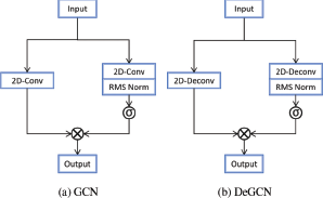
Diagrams of a gated convolutional unit and a gated deconvolutional unit, where σ denotes a sigmoid function.
Diagrams of a gated convolutional unit and a gated deconvolutional unit, where σ denotes a sigmoid function.
The application of LSTM allows modeling long-term dependencies and using deeper layers, but also introduces enormous complexity. However, the efficiency of the model is quite significant for practical applications, for example, the microphone noise reduction program requires efficient computation and a small memory footprint. To mitigate this problem, a grouping strategy is proposed by Gao et al. [6] to improve the model efficiency. The layers of a typical LSTM are fully connected, and the number of inter-layer connections increases dramatically with the number of nodes. As illustrated in Figure 5, the grouping strategy divides the input features and hidden states of each recurrent layer into two groups evenly, and each group processes the internal features independently. In addition, a frame-level rearrangement layer is applied between consecutive recurrent layers to alleviate the problem of the inability to build mutual dependencies between separate groups. And this rearrangement layer brings together distantly-located frames into one group, which potentially allows for learning long-span features. We employ this grouping strategy for the LSTM layers in the proposed dual-branch network and set the number of groups to 2, which is proven to be the most efficient and effective setting in [41].
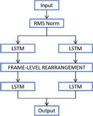
Illustration of a grouped long-short time memory (GLSTM) module.
Illustration of a grouped long-short time memory (GLSTM) module.
3.2 Bridge Module
Figure 6a and 6b show a feature map of the CRN-Time module and the CRN-SRS module, respectively. It can be easily found that their feature maps exhibit distinct patterns, so coarse connections may introduce unnecessary modeling difficulties. Therefore, a bridge module is applied between each convolutional layer from the two branches. The bridge module can be regarded as an information transfer module between different domains, which is responsible for converting information from one branch to another. More specifically, the bridge module is composed of two K × K independent matrices, where K denotes the frame length. Each transformation matrix is trainable and used for a unidirectional transformation process (from the time domain to frequency domain or vice versa). In practical applications, we determine the initial value of the matrix in three ways: random initialization, specific initialization using the real part of fast Fourier transform (FFT) parameters or SRS parameters. We found that initializing the matrix with SRS parameters leads to better performance of the model.
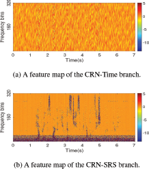
Example feature maps from CRN-TIME and CRN-SRS, they exhibit quite different feature patterns and the values vary widely.
Example feature maps from CRN-TIME and CRN-SRS, they exhibit quite different feature patterns and the values vary widely.
3.3 Feature Normalization
Normalization is a technique to improve generalization ability and facilitate DNN training. Batch normalization [12], layer normalization [1], and instance normalization [42] are widely used for speech enhancement. For a given 4-dimensional input of Batch × Channel × Timeframes × Frequencybins, the three normalization methods calculate the statistics of [B, T, F], [C, T, F] or [T, F] slices respectively, which makes them suitable for different application scenarios. However, we found that the augmentation ability of the network is deprived when the magnitude range of the input is inconsistent with the training samples. In this paper, we propose the feature normalization which can be described as:
where ynorm ∈ ℝB×C×T×F and Ry ∈ ℝB×1×1×F, respectively, are the normalized output and the root mean square of the input data. C and T represent the channels and frames of input data. γ ∈ ℝ1×1×1×F and β ∈ ℝ1×1×1×F are trainable variables of the same size as frequency bins, and + and ⊙ denote element-wise addition and multiplication. e is a small positive constant to avoid division by zero. As described in the formula, we independently compute the root mean square of the input data along the channel and time dimensions for each frequency bin and perform normalization on each frequency bin. In subsequent experiments, we found that feature normalization improves the enhancement ability and still performs well in noise suppression in the face of various untrained amplitude scenarios.
3.4 Time Module And SRS Module
The two branches of the model use the same structure which is similar to CRN. CRN is an encoder-decoder structure composed of convolutional layers and LSTMs, which combines the feature extraction capabilities of CNNs with the temporal modeling capabilities of RNNs. In the proposed network, CRN-Time is fed with time-domain frames of noisy utterances, and CRN-SRS is fed with frequency-domain frames. The encoder stacks 6 normal convolutions with a stride 2 to downsample along the frequency axis, while the decoder stacks 6 deconvolutions with the same stride for upsampling. A modified version of the gated convolutional unit elaborated in Section III. A is used as a convolutional layer, and each one is followed by a parametric ReLU (PReLU) nonlinearity except the output layer. Each layer of the encoder and decoder not only receives the output of the previous layer but also concatenates the corresponding information transformed from the other branch. The used architecture additionally incorporates skip connections to facilitate optimization, which connects each layer in the encoder to its corresponding layer in the decoder. Additionally, we apply the grouping strategy on the intermediate LSTM, which greatly reduces the model complexity.
Table 1 provides a more detailed description of the proposed network architecture. The input size and the output size of each layer are displayed in in Channels × timeFrames × frequencyBins format. The layer hyperparameters are specified in (kernelSize, strides, outChannels) format. For all the convolutions and the deconvolutions, We use a kernel size of 1 × 3 (time × frequency) for the causal system and 3 × 3 for the non-causal system. The number of input channels in each encoder layer is doubled due to the connections of the bridge module, while the number of input channels in the decoder is tripled due to the additional skip connections.
3.5 Loss Functions
The training objective of our dual-branch architecture consists of two parts, corresponding to the outputs generated by these two branches. We employ various loss functions for two outputs to find the best combination. The first loss function is the utterance level mean squared error (MSE) in the time domain which can be defined as:
Architecture of our proposed one branch. Both branches contain the same structure and parameter settings. Here T denotes the number of time frames.
| layer name | input size | hyperparameters | output size |
|---|---|---|---|
| GCN2d_1 | 1 × T × 320 | (1×3), (1,2), 64 | 64 × T × 160 |
| Bridge 1 | 64 × T × 160 | - | 64 × T × 160 |
| GCN2d_2 | 128 × T × 160 | (1×3), (1,2), 64 | 64 × T × 80 |
| Bridge 2 | 64 × T × 80 | - | 64 × T × 80 |
| GCN2d_3 | 128 × T × 80 | (1×3), (1,2), 64 | 64 × T × 40 |
| Bridge_3 | 64 × T × 40 | - | 64 × T × 40 |
| GCN2d_4 | 128 × T × 40 | (1×3), (1,2), 64 | 64 × T × 20 |
| Bridge 4 | 64 × T × 20 | - | 64 × T × 20 |
| GCN2d_5 | 128 × T × 20 | (1×3), (1,2), 64 | 64 × T × 10 |
| Bridge 5 | 64 × T × 10 | - | 64 × T × 10 |
| GCN2d_6 | 128 × T × 10 | (1×3), (1,2), 64 | 64 × T × 5 |
| reshape_1 | 64 × T × 5 | - | T × 320 |
| glstm_1 | T × 320 | 320 | T × 320 |
| glstm_2 | T × 320 | 320 | T × 320 |
| reshape 2 | T × 320 | - | 64 × T × 5 |
| DeGCN2d_6 | 64 × T × 5 | (1×3), (1,2), 64 | 64 × T × 10 |
| Bridge 5 | 64 × T × 10 | - | 64 × T × 10 |
| DeGCN2d_5 | 192 × T × 10 | (1×3), (1,2), 64 | 64 × T × 20 |
| Bridge 4 | 64 × T × 20 | - | 64 × T × 20 |
| DeGCN2d_4 | 192 × T × 20 | (1×3), (1,2), 64 | 64 × T × 40 |
| Bridge_3 | 64 × T × 40 | - | 64 × T × 40 |
| DeGCN2d_3 | 192 × T × 40 | (1×3), (1,2), 64 | 64 × T × 80 |
| Bridge_2 | 64 × T × 80 | - | 64 × T × 80 |
| DeGCN2d_2 | 192 × T × 80 | (1×3), (1,2), 64 | 64 × T × 160 |
| Bridge_1 | 64 × T × 160 | - | 64 × T × 160 |
| DeGCN2d_1 | 192 × T × 160 | (1×3), (1,2), 64 | 64 × T × 320 |
The second one is the mean absolute error loss between the L1 norm of clean and estimated STFT coefficients [32] and can be described as:
where T and F represent the number of time frames and frequency dimensions, S and Ŝ denote STFTs of s and ŝ, respectively. Although LMag obtains better objective scores, it introduces unnecessary artifacts. Therefore, a loss function based LCom on the complex spectrum [49] is applied.
where Sr and Ŝi represent the real and imaginary parts of S, respectively. Finally, we tried three combinations of loss functions: (1)LMse for the time branch, LMag for the frequency branch. (2)LMag for both time- and frequency branch. (3)LCom for both time- and frequency branch. Comparative experiments show that training with the combination (1) can improve the performance of the model, which may indicate that multi-domain constraints are beneficial for model training.
4 Experimental Settings
4.1 Datasets
The proposed dual-branch architecture is evaluated on the WSJ0 SI-84 dataset [35] which includes 7138 utterances from 83 speakers (42 males and 41 females). We select the utterances of 77 speakers (42 males and 41 females) as the original corpus for training and validation sets, while the utterances of the rest 6 speakers (3 males and 3 females) are used to generate the test set. For training, 10000 non-speech sounds from a sound effect library (available at www.sound-ideas.com) [3] are used, and the duration is about 126 h. For testing, we choose two highly challenging noises (babble and cafeteria) from Auditec CD (available at http://www.auditec.com).
During the mixing process, different generative strategies are used for training and testing. For training, we first concatenate all training sentences into one large file and do the same with noises. Then we randomly intercept 7s segments from the speech file and noise file, respectively, and generate mixtures under an SNR uniformly sampled from —5, —4, —3, —2, —1, and —0dB. As a result, a total of 320,000 and 3000 noisy-clean pairs are generated for training and validation, respectively. For testing, 150 utterances from 6 speakers (25 each) are mixed with two selected non-stationary noises at three SNR levels — 5,0, 5 dB. Note that test mixtures are of variable length.
4.2 Experimental Setup
All the utterances are resampled to 16kHz. For SRS operations, Hamming window is used for smoothing. Frame length and frame shift are set to 20ms and 10ms, respectively. For the frame-level operations in the time domain, the 20 ms rectangle window is used to divide each utterance into segments of 320 samples with 50% overlap. All models are developed by PyTorch and trained with stochastic gradient descent optimization using the Adam optimizer [14]. We train the models for 20 epochs with a batch size of 8 at utterance level and keep the learning rate of 0.001. We develop the proposed dual-branch model1 with one NVIDIA RTX 3090 for two weeks.
4.3 Baselines Models
We compared the proposed model with time-domain and frequency-domain methods. In the frequency domain, CRN and GCRN are very representative. As for the time-domain method, we chose AECNN [28], DDAEC [30], and DCN [29] as our baseline methods. The description of baselines is listed as follows:
CRN: it is a convolutional recurrent network in the T-F domain. The network uses 5 convolution layers as the encoder and 5 deconvolution layers as the decoder. Two LSTM layers are used for sequence modeling. This network receives magnitude as input. We kept the best configuration in [40].
GCRN: similar to CRN, it also consists of a convolutional layer and an LSTM with the same structure. The difference is that the GCRN process the signal in the complex domain, and there are two decoders used to recover the real and imaginary parts respectively. Furthermore, a gating mechanism is introduced in the convolutional layers to model more complex interactions, while a grouping strategy is applied to LSTMs to reduce the complexity of the model. We implemented both causal and non-causal versions.
AECNN: it is an autoencoder-based fully convolutional neural network in the time domain. AECNN directly calculates the clean speech segments from the noisy waveform segments. The hyperparameter settings we adopted are consistent with those designed for the WSJ dataset in the original paper.
DDAEC: the network is an encoder-decoder based architecture with skip connections. Layers in the encoder and decoder are followed by densely connected blocks, including dilation and causal convolution. Dilated convolutions are used to aggregate contexts of different resolutions. Subpixel convolution is used in the decoder.
DCN: this is an encoder-decoder based architecture with skip connections. Each layer in the encoder and the decoder comprises a dense block and an attention module. Dense blocks and attention modules help in feature extraction using a combination of feature reuse, increased network depth, and maximum context aggregation. We implemented both causal and non-causal versions. The kernel is set to (1, 3) for the causal system.
4.4 Evaluation Metrics
In our experiments, we use perceptual evaluation of speech quality (PESQ) [36], and short-time objective intelligibility (STOI) [39] as the objective metrics to evaluate the enhancement performance of different models. PESQ is used to evaluate speech quality, with its values ranging from —0.5 to 4.5. STOI values range from 0 to 1, which is used to evaluate speech intelligibility. Note that higher scores for all metrics mean better speech quality.
5 Results, Comparisons and Analyses
5.1 Comparison Results
In this section, we compare the proposed architecture with several excellent baselines and show the results on the WSJ0 SI-84 dataset. Table 2a and Table 2b show the comparison results in terms of the objective metrics STOI and PESQ for two challenging noises at -5 dB, 0 dB, and 5 dB. All the best results are marked in bold in both tables. The proposed dual-branch network (DBCN) yields the best results under all conditions.
For objective metrics, the results in Table 2a and Table 2b show that our proposed models both greatly outperform time-domain DCN and frequency-domain GCRN. Among the frequency-domain baselines, GCRN performs the best. It can achieve an average STOI score of 89.1 and a PESQ score of 2.64 under challenging babble noise. However, the performance of GCRN is far from the proposed method. Compared with the frequency domain, the time-domain method generally has better performance. Among them, the DCN performance is the most prominent. The DBCN still maintains a sufficient advantage in all conditions, especially for the PESQ, which is 0.24 better than DCN on average under babble. In addition to the comparison of causal systems, we provide non-causal versions of GCRN, DCN, and DBCN, denoted GCRN-NC, DCN-NC, and DBCN-NC. In the non-causal version, causal convolutions are replaced by non-causal convolutions, and LSTMs are replaced by bidirectional LSTMs to provide long-term contextual information. The performance of the non-causal system will be significantly improved compared to the causal system because future information is learned. However, we are pleasantly surprised to find that the proposed DBCN outperforms the non-causal system GCRN-NC. This suggests that the proposed model is a highly effective network for speech enhancement even without any context information. We compare DBCN-NC with DCN-NC, the best-performing non-causal baseline system. DBCN-NC obtaine an average improvement of 0.5% and 0.4% for babble and cafeteria in terms of STOI, respectively, and an average improvement of 0.06 and 0.09 for PESQ.
Evaluations and comparisons of different enhancement models in terms of STOI(%).
| Metrix | STOI | Casual? | |||||||
|---|---|---|---|---|---|---|---|---|---|
| Test Noise | Babble | Cafeteria | |||||||
| Test SNR (dB) | -5 | 0 | 5 | Avg. | -5 | 0 | 5 | Avg. | |
| Mixture | 58.5 | 70.4 | 81.2 | 70.0 | 57.5 | 69.9 | 81.1 | 69.5 | |
| CRN | 77.9 | 88.0 | 93.2 | 86.4 | 75.7 | 86.6 | 92.7 | 85.0 | ✓ |
| GCRN | 81.5 | 90.8 | 94.9 | 89.1 | 78.5 | 89.0 | 94.3 | 87.3 | ✓ |
| AECNN | 80.5 | 90.6 | 94.2 | 88.4 | 80.0 | 89.4 | 94.0 | 87.8 | ✓ |
| DDAEC | 84.0 | 92.2 | 95.6 | 90.6 | 81.7 | 90.9 | 94.9 | 89.2 | ✓ |
| DCN | 83.9 | 91.8 | 95.2 | 90.3 | 81.0 | 90.3 | 94.5 | 88.6 | ✓ |
| DBCN | 85.3 | 92.7 | 95.9 | 91.3 | 82.0 | 91.2 | 95.2 | 89.5 | ✓ |
| GCRN-NC | 84.1 | 92.1 | 95.5 | 90.5 | 81.3 | 90.5 | 95.0 | 89.0 | ✕ |
| DCN-NC | 87.9 | 93.5 | 96.1 | 92.5 | 85.0 | 92.1 | 95.3 | 90.8 | ✕ |
| DBCN-NC | 88.3 | 94.1 | 96.5 | 93.0 | 85.2 | 92.5 | 96.0 | 91.2 | ✕ |
Evaluations and comparisons of different enhancement models in terms of PESQ.
| Metrix | PESQ | Casual? | |||||||
|---|---|---|---|---|---|---|---|---|---|
| Test Noise | Babble | Cafeteria | |||||||
| Test SNR (dB) | -5 | 0 | 5 | Avg. | -5 | 0 | 5 | Avg. | |
| Mixture | 1.54 | 1.82 | 2.12 | 1.83 | 1.46 | 1.77 | 2.12 | 1.78 | |
| CRN | 1.99 | 2.50 | 2.91 | 2.47 | 2.01 | 2.47 | 2.89 | 2.46 | ✓ |
| GCRN | 2.08 | 2.71 | 3.13 | 2.64 | 2.03 | 2.62 | 3.09 | 2.58 | ✓ |
| AECNN | 2.00 | 2.57 | 2.88 | 2.48 | 2.03 | 2.55 | 2.93 | 2.50 | ✓ |
| DDAEC | 2.33 | 2.88 | 3.26 | 2.82 | 2.30 | 2.81 | 3.19 | 2.77 | ✓ |
| DCN | 2.23 | 2.72 | 3.09 | 2.68 | 2.15 | 2.62 | 3.01 | 2.59 | ✓ |
| DBCN | 2.45 | 2.98 | 3.33 | 2.92 | 2.29 | 2.84 | 3.24 | 2.79 | ✓ |
| GCRN-NC | 2.22 | 2.81 | 3.17 | 2.73 | 2.08 | 2.72 | 3.07 | 2.62 | ✕ |
| DCN-NC | 2.61 | 3.04 | 3.33 | 2.99 | 2.45 | 2.91 | 3.23 | 2.86 | ✕ |
| DBCN-NC | 2.63 | 3.12 | 3.38 | 3.05 | 2.48 | 3.01 | 3.35 | 2.95 | ✕ |
In conclusion, the proposed dual-branch model outperforms both DCN which is a time-domain based model, and GCRN which is a frequency-domain based model for complex spectrogram mapping, indicating that information transformation and fusion of two domains can significantly improve the performance of the model and improve parameter utilization.
5.2 Ablation Study
In this section, we conduct ablation experiments on various constituent techniques of the causal system. As shown in Table 3, we evaluate the contributions of the components by taking the average of all test results. “- FN” means that we remove the feature normalization and use the batch normalization instead. “-BG” means to use random values to initialize the weight matrices in the bridge layer instead of the SRS coefficients. CRN-Time and CRN-SRS stands for single-branch on time and frequency domain respectively. For fair comparison, we adjusted all systems to have similar numbers of parameters.
We can find that all the variants underperforms the proposed dual-branch architecture, regardless of whether the feature normalization or bridge modules are replaced. Among them, feature normalization plays a more important role, which brings 1.0% STOI and 0.19 PESQ improvement under the babble condition. Note that replacing the bridge layer initialization method is not equivalent to deleting the bridge layer, but using a random initialization method. Under babble condition, STOI attenuates by 0.4% and PESQ attenuates by 0.12. Additionally, two independent single-branch variants were also evaluated. We can find that missing the reference information from the other branch leads to a sharp drop in performance. The independent time-domain branch and the frequency-domain branch reduce STOI by 3.4% and 3.7% under the babble, respectively. It further proves that the dual-branch network improves the enhancement performance by using alternate interconnection.
5.3 Comparison of Loss Function
To analyze the effectiveness of the loss function, we compare the models trained using different loss functions. First, we apply utterance-level MSE constraints to the time-branch outputs and magnitude-spectral constraints to the frequency-domain outputs, which are denoted as “LMse-LMag”. Second, the magnitude spectral constraint is imposed on both outputs simultaneously, denoted as “LMag-LMag”. These two combinations are used to prove that the combination of different domain loss functions benefits the performance of the dual-branch network. However, the used LMag loss function brings unknown artifacts to the enhanced speech, which corrupts the subjective perception. Therefore, the complex loss, which constrains both real and imaginary components and magnitude, is used on both outputs to alleviate this problem. This is denoted as “LCom-LCom”.
Evaluations and comparisons of models using different loss function in terms of STOI(%). The best socre is marked in bold.
| Metrix | STOI | |||||||
|---|---|---|---|---|---|---|---|---|
| Test Noise | Babble | Cafeteria | ||||||
| Test SNR (dB) | -5 | 0 | 5 | Avg. | -5 | 0 | 5 | Avg. |
| LMse-LMag | 85.3 | 92.7 | 95.9 | 91.3 | 82.0 | 91.2 | 95.2 | 89.5 |
| LMag-LMag | 84.8 | 92.3 | 95.6 | 90.9 | 81.4 | 90.6 | 95.0 | 88.6 |
| LCom-Lcom | 84.5 | 92.3 | 95.6 | 90.8 | 80.6 | 90.4 | 95.1 | 88.3 |
| LMse-LMag-NC | 88.6 | 94.1 | 96.5 | 93.1 | 85.2 | 92.5 | 96.0 | 91.2 |
| LMag-LMag-NC | 88.6 | 94.2 | 96.5 | 93.1 | 85.1 | 92.5 | 96.0 | 91.2 |
| Lcom-Lcom-NC | 88.3 | 94.1 | 96.5 | 93.0 | 84.6 | 92.3 | 96.0 | 91.0 |
Evaluations and comparisons of models using different loss function in terms of PESQ. The best socre is marked in bold.
| Metrix | PESQ | |||||||
|---|---|---|---|---|---|---|---|---|
| Test Noise | Babble | Cafeteria | ||||||
| Test SNR (dB) | -5 | 0 | 5 | Avg. | -5 | 0 | 5 | Avg. |
| LMse-LMag | 2.45 | 2.98 | 3.33 | 2.92 | 2.29 | 2.84 | 3.24 | 2.79 |
| LMag-LMag | 2.32 | 2.85 | 3.21 | 2.79 | 2.15 | 2.72 | 3.15 | 2.67 |
| LCom-Lcom | 2.24 | 2.85 | 3.25 | 2.78 | 2.04 | 2.68 | 3.19 | 2.64 |
| LMse-LMag-NC | 2.63 | 3.12 | 3.38 | 3.05 | 2.48 | 3.01 | 3.35 | 2.95 |
| LMag-LMag-NC | 2.64 | 3.13 | 3.38 | 3.05 | 2.47 | 3.00 | 3.35 | 2.94 |
| Lcom-Lcom-NC | 2.65 | 3.15 | 3.45 | 3.08 | 2.45 | 3.02 | 3.41 | 2.96 |
Table 4a and Table 4b gives the comparison results for the three combinations. For the causal system, the combination of LMse-LMag consistently outperforms the other loss functions in all conditions. It is the deviation of the two learning objectives that makes the features extracted by the two branches more differentiated, prompting each branch to focus on the noise it excels and reducing the learning difficulty of individual branches. Then, the transformation and fusion of the bridge layers allow the information to complement each other, giving a huge boost to the model performance. In contrast, in the non-causal system, the combination of LMse and LMag still maintains the advantage in STOI, but lags behind LCom in PESQ, especially at high signal-to-noise ratios. It can be noticed that the frequency domain branch using LMag lacks the phase constraint compared to LCom, which suggests that the extra phase constraint could bring improvement in speech quality when the contextual information is sufficient.
Table 4a and Table 4b shows the results of the three combinations, and it can be seen that the combination of constraints in different domains can bring performance improvements. In our records, however, the performance of the time branch drops considerably. We reckon that it is the deviation of the learning target of the two branches that makes the information from the other branch more instructive, resulting in better performance of the frequency domain branch. Additionally, we notice that LMag does not consistently improve PESQ at different SNRs. At low SNR, LCom obtains better performances than the others. Consistent with the previously mentioned, we think this is because LMag introduces artifacts and PESQ is more sensitive to artifacts. Moreover, this problem is more pronounced in non-causal systems. According to the results, the combination of LMse and LMag may be the best choice.
5.4 Comparison of Model Complexities
The number of parameters and computational complexity are important indicators for evaluating a model and determining the scenarios in which the model can be applied. We evaluate the model complexity of the proposed model and other baseline systems using trainable parameters and memory access cost (MAC) for processing one second of speech. As shown in the Table 5, the dual-branch model has about 2.85M parameters and 6.12G MAC per second signal. Compared with the frequency domain model, the proposed model has a bit more computational cost and fewer trainable parameters, while the performance of the model is much better than the baseline in the frequency domain. Compared with the time-domain model, the proposed model is superior in terms of parameter quantity, computational complexity, and even performance. This undoubtedly proves the effectiveness of the dual branch network.
6 Conclusion
In this study, we propose a novel dual-path convolutional network for cross-domain speech enhancement, where the time-domain branch pays more attention to local information, and the frequency-domain branch pays more attention to the relationship between frames. The bridge layer is introduced for the conversion and fusion of information between the two domains, thus the two branches can achieve the effect of mutual guidance. Furthermore, we propose a novel feature normalization method. The relative relationship between frames of each frequency point can be obtained by using statistical root mean square to regulate data. In the absence of bias, the model maintains complete noise reduction capability for input waveform with arbitrary amplitudes.
We have developed causal and non-causal DBCN, which are trained on the WSJ corpus and evaluated on untrained WSJ speakers. Systematic comparison experiments and ablation experiments of each module are conducted, which proved that DBCN outperforms existing noise and speaker-independent approaches for speech enhancement. In addition, the amount of parameters and computation of the proposed network is much smaller than other time-domain baselines, and it can denoise under fully causal conditions. However, due to equipment limitations, this algorithm cannot be applied to terminal equipment. In future studies, we will design more suitable structures for each domain and plan to further reduce the computational load of the model to better implement the algorithm in real time scenarios. Finally, we consider introducing a pre-training strategy to improve the practicality and performance of the model.
This research was supported by the China National Nature Science Foundation (No. 61876214). This work was also supported by The Project (KF-2022-07-009) Supported the Open Fund of Key Laboratory of Urban Land Resources Monitoring and Simulation, Ministry of Natural Resources, China.
The code and examples: https://github.com/zhangkanghao/DBCN.

