


Proximal splitting-based convex optimization is a promising approach to linear inverse problems because we can use some prior knowledge of the unknown variables explicitly. An understanding of the behavior of the optimization algorithms would be important for the tuning of the parameters and the development of new algorithms. In this paper, we first analyze the asymptotic property of the proximity operator for the squared loss function, which appears in the update equations of some proximal splitting methods for linear inverse problems. Our analysis shows that the output of the proximity operator can be characterized with a scalar random variable in the large system limit. Moreover, we apply the asymptotic result to the prediction of optimization algorithms for compressed sensing. Simulation results demonstrate that the MSE performance of the Douglas-Rachford algorithm can be well predicted in compressed sensing with the ℓ1 optimization. We also examine the behavior of the prediction for the case with nonconvex smoothly clipped absolute deviation (SCAD) and minimax concave penalty (MCP) regularization.
1 Introduction
Linear inverse problems, i.e., the reconstruction of an unknown vector from its linear measurements, often appear in the field of signal processing. The linear inverse problem is called underdetermined when the number of measurements is less than that of elements of the unknown vector. In such underdetermined problems, we often use some information about the unknown vector to obtain a good reconstruction result. In compressed sensing [8, 7, 16, 9], for example, the unknown sparse vector can be effectively reconstructed by leveraging its sparsity. Another example of the underdetermined problems is the overloaded signal detection in wireless communications [33, 23, 24], where we can use the discreteness of the unknown vector.
A common approach to underdetermined linear inverse problems is to solve an optimization problem using some regularizer based on the prior knowledge of the unknown vector. In compressed sensing, one of the most widely used optimization problems is the ℓ1 optimization. The objective function includes the ℓ1 regularization term to promote sparsity. Even though the objective function is not differentiable because of the ℓ1 norm, some proximal splitting methods can solve the problem with reasonable computational complexity. Examples of such methods include the iterative soft thresholding algorithm (ISTA) [15, 14, 21] and the fast ISTA (FISTA) [5]. Alternating direction method of multipliers (ADMM) [22, 6] and the Douglas-Rachford algorithm [28, 19, 13] can both be used to solve the ℓ1 optimization problem. Despite the requirement of matrix inversion for linear inverse problems, ADMM and the Douglas-Rachford algorithm exhibit faster convergence than some gradient-based methods, such as ISTA, in certain cases [11, 12].
The asymptotic error performance of several optimization-based approaches for linear inverse problems has been analyzed by using some techniques [18, 3, 17]. Especially, the convex Gaussian min-max theorem (CGMT) [36, 35] enables us to obtain the asymptotic error in a precise manner for the optimizer of various optimization problems. For instance, the asymptotic mean-square-error (MSE) of various regularized estimators has been analyzed in [2, 35]. In [37, 27], the symbol error rate has also been analyzed for the reconstruction of discrete-valued vectors.
The above analyses have focused on the performance of the optimizer, whereas the application of CGMT for the performance prediction of optimization algorithms has been considered in [26]. In [26], we have proposed a prediction method for the error performance of the tentative estimate at each iteration of ADMM. Such performance prediction could be utilized to understand the behavior of the algorithm, tune the parameter, and develop a new algorithm. For optimization algorithms other than ADMM, however, such asymptotic performance prediction has not been discussed for linear inverse problems in the literature. Expanding the prediction method to other optimization algorithms would be important for the development of new algorithms and the understanding of the behavior of the algorithms.
In this paper, we investigate the asymptotic behavior of algorithms using the proximity operator of the squared loss function. As the target optimization problem, we consider the objective function with the squared loss function and a separable regularizer. Since the proximity operator of the squared loss function is not element-wise, we investigate its asymptotic property via the CGMT framework. Our main finding is that the optimization problem in the definition of the proximity operator can be analyzed by using CGMT for the squared loss function. Specifically, we show that the output of the proximity operator for the squared loss function can be regarded as a scalar random variable in the large system limit.
By using the analytical result, we also propose a prediction method for the evolution of the asymptotic MSE in proximal splitting methods composed of the proximity operator of the squared loss function and a separable reg-ularizer. As an representative example of such algorithms, we here consider the Douglas-Rachford algorithm in this paper. While the derivation of the proposed method is partly non-rigorous, their simulation results for the ℓ1 optimization demonstrate their potential as a foundation for more rigorous discussion in future work. These findings would contribute to the broader understanding of optimization algorithms in high-dimensional settings. Moreover, we also investigate the behavior for the case with nonconvex regularization in the simulation, though only the convex optimization is considered in [26]. The effectiveness of the performance prediction across various scenarios highlights its potential to extend to other optimization algorithms, including those involving nonconvex cases.
We use the following notations in this paper. The transpose and the identity matrix are denoted by (·)⊤ and I, respectively. The ℓ1 norm and the ℓ2 norm for a vector u = [u1 ⋯ uN]⊤ ∈ ℝN are defined as and , respectively. We denote the sign function by sign(·). For a lower semicontinuous function ϕ: ℝN → ℝ ⋃ {+∞}, the proximity operator is defined as . We denote the Gaussian distribution with mean μ and variance σ2 by 𝓝(μ, σ2). If random variables {Θn} (n = 1, 2, …) with index n converge in probability to Θ, we use the notation as n → ∞ or plimn→∞ Θn = Θ.
2 Optimization for Linear Inverse Problems
2.1 Linear Inverse Problems
In this paper, we discuss the linear inverse problem, which means the reconstruction of a vector x ∈ ℝN from its measurement y ∈ ℝM given by
The measurement matrix A ∈ ℝM × N is assumed to be known and v ∈ ℝM denotes a noise vector. We mainly focus on the underdetermined case where the measurement ratio Δ := M/N is less than 1 and the solution is not unique even in the noiseless case. A common approach in this situation is the utilization of the structure of x. In compressed sensing, for example, the unknown vector is assumed to be sparse, i.e., the vector has many zero elements. In some applications in wireless communications, the unknown vector has other structures such as boundedness and discreteness [34, 30, 1, 25].
2.2 Optimization-Based Approach
Mathematical optimization is a useful method for underdetermined linear inverse problems. In this approach, we can design the objective function of the problem to make the most of the structure of the unknown vector x. As a simple example, we discuss the following optimization problem
in this paper. We refer to as the squared loss function. The function fλ(·): ℝN → ℝ ⋃ {+∞} is a regularizer that can incorporate prior knowledge of the unknown vector x. The parameter λ determines the balance between two terms in the objective function.
In the sparse vector reconstruction, for example, the ℓ1 regularization by fλ(s) = λ||s||1 (λ > 0) is widely used as a convex regularizer. The elastic net [40] given by , where λ1,λ2 (> 0) are the parameters, is also a popular convex regularizer. Other than these convex regulariz-ers, various nonconvex regularizers have been proposed for the sparse vector reconstruction [38]. For example, the smoothly clipped absolute deviation (SCAD) [20] regularizer is given by , where
and a(> 1) is the parameter. For the minimax concave penalty (MCP) [391 regularizer, the function is given by
where b (> 0) is the parameter.
Various optimization algorithms have been proposed for the optimization problem in (2). For example, the Douglas-Rachford algorithm [28, 19, 13| solves the optimization problem in (2) by using the proximity operators of L(·) and fλ(·). The update equations of the algorithm with the iteration index k (=0, 1, 2, …) can be written as
where γ(> 0) and ρk ∈ [ε, 2 − ε] (ε ∈ (0, 1)) are the parameters in the algorithm. By definition, we can obtain the proximity operator of the function L(·) as
where z ∈ ℝN and γ > 0. The proximity operator of fλ(·) can also be computed efficiently for various regularizers. When fλ(s) = λ ||s||1 for example, the proximity operator of the function fλ(·) can be written as
where rn and are the n-th element of r and , respectively. For the elastic net regularizer , the proximity operator can be computed as
As for the SCAD regularizer in (3), the proximity operator is given by
for a > 1 + γ. Similarly, the proximity operator of the MCP regularizer in (4) can be computed as
for b > γ. By computing (5) and (6) iteratively, we can obtain a sequence {s(k)} k=1,2, … converging to the solution of the optimization problem in (2) when the regularizer is convex. When the regularizer is nonconvex, the convergence of the sequence is not necessarily guaranteed.
3 Main Results
3.1 Asymptotics of Proximity Operator for Squared Loss
We firstly analyze the output of the proximity operator proxγL(·) in (8). In our analysis, we assume the large system limit M,N → ∞ (M/N = Δ), where the sequence of problems with {x, A, v} indexed by N is considered as in several high-dimensional analyses [35]. We also assume the following conditions as in [26].
Assumption 3.1. The elements of the vector x ∈ ℝN are independent and identically distributed (i.i.d.). The distribution pX of x is known and has some finite mean and variance. The measurement matrix A ∈ ℝM × N has i.i.d. random variables with 𝓝(0, 1/N). The noise vector v ∈ ℝM has i.i.d. random variables with .
Remark 3.1. We assume that each element of the measurement matrix A follows a Gaussian distribution in Assumption 3.1. This is because we require the Gaussian assumption in the analysis with CGMT [35]. Nonetheless, the universality of random matrices discussed in [4, 32, 31] implies that the analytical result still holds for some other distributions. In [35, Section VIII-F], for example, it is expected that the analysis via CGMT holds for i.i.d. sub-Gaussian matrix. Computer simulations in [35, 26] show that the empirical performance is well predicted even when the measurement matrix is composed of i.i.d. Bernoulli distribution with p = 0.5.
Under Assumption 3.1, we can obtain the following result on the asymptotic behavior of the proximity operator proxγL(·).
Proposition 3.1. It is assumed that x, A, and v satisfy the conditions in Assumption 3.1. We then consider the output of the proximity operator given by
where z has i.i.d. elements with a distribution pZ(z) and is assumed to be independent of A. Here, we assume that the optimization problem
has a unique optimizer (α*,β*)1. In (14),
X ~ PX, H ~ 𝓝(0, 1), and Z ~ pZ. The expectation E [·] in (14) is calculated over all random variables X, H, and Z. Then, the following statements hold:
1. The asymptotic MSE of ŝ in (13) can be written as
2. Let μg denote the empirical distribution of ŝ = [ŝ1 … ŝN]⊤ ∈ ℝN that corresponds to the cumulative distribution function (CDF) given by , where 𝕀 (ŝn< s) = 1 if ŝn< s and otherwise 𝕀 (ŝn< s) = 0. Then, the distribution μg converges weakly in probability to the distribution μS of S = Ŝ (α*, β*; Z), i.e., holds for any continuous compactly supported function g(·): ℝ → ℝ.
Sketch of proof. By definition in (13), ŝ is characterized as the solution of the optimization problem in (7). Similarly to the discussion in [27, Remark IV.1], we can prove (17) by using the standard method with CGMT [35]. Moreover, the second statement of Proposition 3.1 is proven in the procedure of [27, Theorem III.2]. Hence, we do not include the details of the rigorous proof. For the overview of the derivation of (14), see Appendix A.1. □
The first statement in Proposition 3.1 means that the asymptotic MSE for the output of the proximity operator can be predicted by solving the scalar optimization problem in (14). The second one implies that the distribution of the elements of the vector ŝ can be characterized by the random variable S = Ŝ (α*, β*; Z). We can thus consider Ŝ (α*, β*; Z) in (16) as a decoupled version of the proximity operator in (13) intuitively. For a similar discussion, see [26, Fig. 1].
The optimization of α and β in (14) can be performed by using searching methods like the golden section search [29]. Since it is difficult to compute the expectation in (14) exactly in general, we need to approximate it with the average of many realizations of X, H, and Z.
3.2 Application to Performance Prediction of Optimization Algorithm
Although the proximity operator itself is not a valid reconstruction method in general, we believe that the result in Proposition 3.1 is not only of theoretical interest but also serves as a foundation for understanding and designing optimization algorithms in linear inverse problems. By using Proposition 3.1, for example, we can derive an error prediction method for the estimate s(k) in some optimization algorithm. To obtain the prediction method, we make an additional assumption that the regularizer fλ(·) is convex and separable as follows.
Assumption 3.2. The function fλ(·) : ℝN → ℝ ⋃ {+∞} is separable and can be written as with a convex function . We sometimes use the notation ƒλ(·) for the corresponding function with the slight abuse of notation.
Remark 3.2. For the separable regularizer ƒλ(·) in Assumption 3.2, the proximity operator proxγƒλ (·): ℝN → ℝN becomes an element-wise function. In other words, the n-th element of the output of the proximity operator is the function of the n-th element of the input only.
To predict the performance of an algorithm by using Proposition 3.1, it is necessary that the update equations except for proxγL(·) are element-wise. As a representative example of such algorithms, we derive the conjecture below for Douglas-Rachford algorithm in (5) and (6). Note that the derivation of the conjecture is partly non-rigorous as [26, Claim III.1].
Conjecture 3.1. Suppose that Assumptions 3.1 and 3.2 hold. We define the stochastic process
with the index k. We here assume that the optimization problem
has a unique optimizer (α*k, β*k). Then, we have the following conjecture:
1. The asymptotic MSE of s(k+1) in (5) can be written as
2. The empirical distribution of s(k+1) converges weakly in probability to the distribution of Sk+1.
Outline of derivation. Since z(k) in (5) and (6) is not independent of A, Proposition 3.1 cannot be used to (5) directly. We thus take the same procedure as the approach in [26, Claim III.1], where an unproven extension of CGMT has been assumed for the performance prediction of iterative algorithms. Under the assumption, when the element of z(k) can be regarded as the random variable Zk, the distribution of the element of s(k+1) in (5) can be described by the distribution of the random variable Sk+1 in (18) as in Proposition 3.1. As for (6), the update of z(k) can be decoupled into (19) because the update is element-wise under Assumption 3.2. Since the procedure of the derivation is the same as [26, Claim III.1], the detailed explanation for the derivation is omitted. □
Conjecture 3.1 implies that the evolution of the asymptotic MSE in the Douglas-Rachford algorithm can be predicted by solving the optimization problem in (20) and computing (21) for each k. The updates of Sk and Zk in (18) and (19) can be seen as a simplified version of the update of s(k) and z(k) in (5) and (6), respectively.
From the result in Conjecture 3.1, we can tune the parameters in the Douglas-Rachford algorithm for fast convergence. Since the relation between the parameters and the MSE is complicated, it is difficult to obtain the explicit expression of the optimal parameters. However, the result enables us to predict the error performance of the algorithm numerically and to select the parameter that achieves fast convergence in the asymptotic regime, without the empirical reconstruction.
Remark 3.3. As discussed in [19], the Douglas-Rachford algorithm is closely related to ADMM analyzed in [26]. In fact, the update equations of ADMM can be regarded as the Douglas-Rachford algorithm for the dual problem of the original optimization problem. However, the relaxation parameters ρk are included in the Douglas-Rachford algorithm considered in this paper, whereas the corresponding parameters are not considered in the analysis of [26]. These parameters provide additional flexibility in tuning the algorithm for faster convergence. Furthermore, since we have expressed Proposition 3.1 as the result for the proximity operator for the squared loss function, our results have the potential to be extended to other optimization algorithms that utilize the proximity operator.
4 Simulation Results
In this section, we demonstrate the validity of our approach via computer simulations. The distribution of an unknown vector x is assumed to be the Bernoulli-Gaussian distribution given by
Here, δ0(·) is the Dirac delta function, pH (·) is the probability density function corresponding to 𝒩(0, 1), and p0 ∈ (0, 1) represents the probability of 0. The unknown vector x is sparse when p0 is large. For the simulations, we assume that the measurement matrix A and the noise vector v satisfy the conditions in Assumption 3.1 unless otherwise stated. For the optimization of α and β in (14) and (20), the golden section search is used.
4.1 MSE of Output of Proximity Operator for Squared Loss
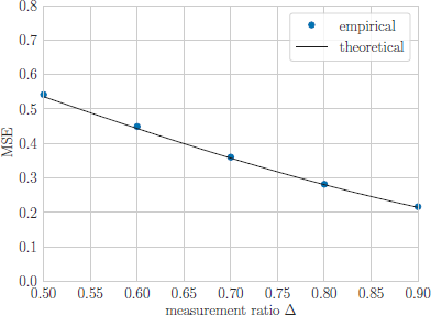
We demonstrate a simulation result for the first statement of Proposition 3.1. In Figure 1, the empirical MSE of ŝ = proxγL(z) in (13) is compared with the corresponding theoretical prediction in (17). In the simulation, we set , and γ = 10. In the figure, ‘empirical’ denotes the empirical MSE of ŝ and ‘theoretical’ denotes the corresponding asymptotic value . For the computation of the empirical MSE, we first make the realizations of x, A, and ν to compute y from (1). We then create each element of z from the i.i.d. standard Gaussian distribution. Using these realizations, we compute the MSE of ŝ from (8) and (13). The empirical performance in the figure is obtained by averaging the MSE for 100 independent realizations. For the theoretical prediction, we solve the scalar optimization problem in (14) to obtain a*. Note that we approximate the expectation in the optimization problem with 100,000 realizations of X ~ pX, H ~ 𝒩(0, 1) and Ζ ~ 𝒩(0, 1). From Figure 1, we observe that the empirical performance and its theoretical prediction agree well with each other for various measurement ratios Δ.
4.2 Distribution of Output of Proximity Operator for Squared Loss
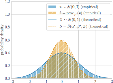
We then examine the second statement of Proposition 3.1. In Figure 2, we compare the probability density of the elements of ŝ = proxγL(z) with the theoretical result. In the simulation, we set , and γ = 10. The empirical ŝ = proxγL(z) and the realizations of the corresponding random variable S = Ŝ (α*, β*; Ζ) is obtained in the same way as the first experiment. The empirical histogram is obtained from the result of 100 independent trials. From Figure 2, we can see that the empirical distribution of ŝ agrees well with the distribution of S obtained by Proposition 3.1.
4.3 Performance Prediction of Douglas-Rachford Algorithm with Convex Regularization
Next, we investigate the validity of Conjecture 3.1. For the reconstruction of the sparse vector following (22), we first consider the ℓ1 optimization with fλ(s) = λ ||s||1, i.e.,
which is a widely used convex optimization problem in compressed sensing and satisfies Assumption 3.2. For the ℓ1 regularization, the proximity operator is given by (9).
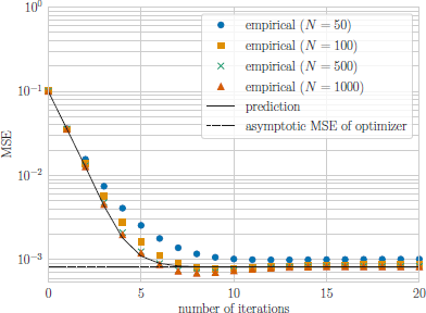
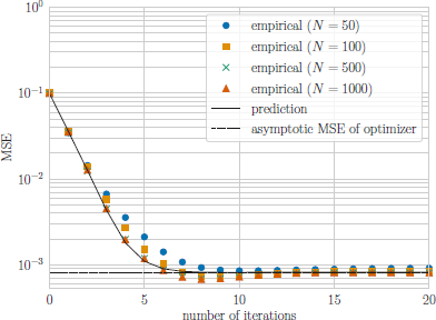
We compare the empirical MSE performance of the Douglas-Rachford algorithm for (23) and its prediction obtained from Conjecture 3.1. In Figure 3, we show the MSE performance versus the number of iterations in the algorithm, where Δ = 0.7, p0 = 0.9, and . The parameters of the Douglas-Rachford algorithm are set as γ =10 and ρk = 1. The initial values of s(k) and z(k)are given by s(0)= z(0) = 0. In Figure 3, ‘empirical’ refers to the empirical MSE performance of the Douglas-Rachford algorithm in (5) and (6). The MSE curve is the average of the performance for 500 independent realizations of the reconstruction problem. Also, ‘prediction’ represents the predicted MSE obtained by Conjecture 3.1. To calculate the prediction, we compute (a*k,β*k) and 100,000 realizations of (Sk, Zk) for k = 0,1, … from (18) and (19), following the similar way to [26]. Here, the expectation in (20) is approximated by using the realizations of (Sk, Zk). In Figure 3, we also show the asymptotic MSE of the optimizer of (23) as ‘asymptotic MSE of optimizer,’ which is derived by using the standard CGMT approach [35]. The value of the parameter λ in (23) is selected to minimize the asymptotic MSE of the optimizer. Figure 3 shows that the empirical performance is close to the prediction when Ν is sufficiently large. We can also see that they approach the asymptotic MSE of the optimizer after sufficient iterations. To be precise, however, we can observe a slight difference between the prediction and the empirical performance. This is partly because we evaluate the empirical performance for finite N, while we assume M, N→∞to obtain the asymptotic prediction. Another possible reason is that we approximate (a*k,ß*k) by using many realizations of (Sk, Zk) in the prediction.
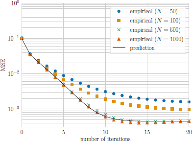
We also investigate the performance of the Douglas-Rachford algorithm with the elastic net regularization in Figure 4. In the simulation, we set , and pk = 1. As in the case with the ℓ1 regularization, the empirical performance is well predicted by the prediction when Ν is sufficiently large.
MSE performance of Douglas-Rachford algorithm with elastic net regularization .
MSE performance of Douglas-Rachford algorithm with elastic net regularization .
Figure 5 shows the MSE performance of the Douglas-Rachford algorithm with the ℓ1 regularization for the Bernoulli measurement matrix. In the evaluation of the empirical performance, the element of the measurement matrix A ∈ ℝΜ × N is generated from the i.i.d. distribution given by , where am, n denotes the (m, n) element of A. For other parameters, we set the same values as in Figure 3. From Figure 5, we can see that the empirical performance is well predicted by the prediction even for the Bernoulli measurement matrix, though the Gaussian measurement matrix is assumed in derivation of the prediction.
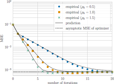
Figure 6 shows the MSE performance of the Douglas-Rachford algorithm with the ℓ1 regularization for different values of pk. In the figure, the parameters are , and γ = 5.0. From the figure, we observe that the empirical performance is well predicted for every different values of pk. We can also see that the convergence speed is significantly influenced by the value of pk.
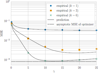
We then show the MSE performance of the Douglas-Rachford algorithm with the ℓ1 regularization for different parameters γ in Figure 7. In the figure, we have , and pk = 1. From the figure, we can observe that the performance is improved as the iteration index k increases. The figure also implies that the value of γ significantly affects the performance of the algorithm. Since the empirical performance is well predicted for all γ, we can tune the parameter by using the prediction. The figure shows that we should choose γ between 10 and 15 in this case.
MSE performance of Douglas-Rachford algorithm for ℓ1 optimization (Bernoulli measurement matrix, .
MSE performance of Douglas-Rachford algorithm for ℓ1 optimization (Bernoulli measurement matrix, .
We also investigate the performance of the Douglas-Rachford algorithm with the ℓ1 regularization for different values of in Figure 8. In the figure, we set Ν = 500, Δ = 0.7, p0 = 0.9, γ = 10, and pk = 1. From Figure 8, we can see that the empirical performance is well predicted for different values of . The figure also implies that the performance is improved as the value of decreases, though the required number of iterations for the convergence increases.
4.4 Performance Prediction of Douglas-Rachford Algorithm with Non-convex Regularization
Finally, we evaluate the performance for nonconvex sparse regularization. Figure 9 shows the MSE performance of the Douglas-Rachford algorithm with SCAD regularization in (3), where , and a = 4. The empirical performance and the prediction are obtained in the same way as Figure 3. From Figure 9, we observe that the empirical MSE and its prediction converge to almost the same value in this case. In the middle of iterations, however, the behavior of the prediction is different from Figure 3, and the empirical performance when Ν = 500, 1000 is better than the prediction. One of the possible reasons is the nonconvexity of the SCAD regularizer, and further investigation is necessary for a clear understanding. To obtain more precise results, we might need to taking the nonconvexity into account in the analysis.
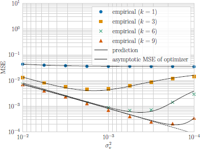
MSE performance of Douglas-Rachford algorithm for ℓ1 optimization versus {N = 500, Δ = 0.7, p0 = 0.9, γ = 10, pk = 1).
MSE performance of Douglas-Rachford algorithm for ℓ1 optimization versus {N = 500, Δ = 0.7, p0 = 0.9, γ = 10, pk = 1).
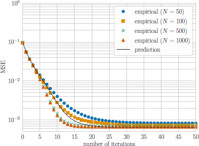
MSE performance of Douglas-Rachford algorithm with nonconvex SCAD regularization .
MSE performance of Douglas-Rachford algorithm with nonconvex SCAD regularization .
We also investigate the performance of the Douglas-Rachford algorithm with SCAD regularization for a larger noise variance in Figure 10, where Δ = 0.7, p0 = 0.9, λ = 0.2, γ = 1, pk = 1, and a = 4. From the figure, we can see that the empirical performance is well predicted in this case. The difference in behavior compared to Figure 9 is probably influenced by the value of and other parameters, presenting an intriguing avenue for future research.
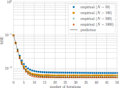
Figure 11 shows the performance of the Douglas-Rachford algorithm with the nonconvex MCP regularization. In the simulation, we set , and b = 4. As in Figure 9, the empirical performance when Ν = 500, 1000 is better than the prediction in the middle of iterations. These results suggest that the nonconvexity of the MCP regularizer also affects the behavior of the prediction.
Figure 12 shows the MSE at the 50-th iteration versus the regularization parameter λ, where , and pk = 1. In the simulation, we use the SCAD regularization with a = 4. From the figure, we can see that the prediction is close to the empirical performance for λ ≥ 0.08, whereas the prediction is worse for smaller values of λ. Even in this case, however, we can tune a reasonable value of λ ≈ 0.07 on the basis of the prediction, without the empirical reconstruction.
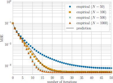
MSE performance of Douglas-Rachford algorithm with nonconvex MCP regularization .
MSE performance of Douglas-Rachford algorithm with nonconvex MCP regularization .
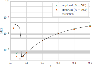
MSE performance of Douglas-Rachford algorithm with nonconvex SCAD regularization versus .
MSE performance of Douglas-Rachford algorithm with nonconvex SCAD regularization versus .
5 Conclusion
In this paper, we have analyzed the asymptotic behavior of the proximity operator for the squared loss function in linear inverse problems. We have also shown that the result in Proposition 3.1 can be used for the asymptotic performance prediction of some optimization algorithms for large-scale linear inverse problems. Simulation results show that the empirical distribution of the output of the proximity operator agrees well with the theoretical prediction by Proposition 3.1. Moreover, the empirical MSE performance of the Douglas-Rachford algorithm can be well predicted in large-scale compressed sensing via the ℓ1 optimization. For the nonconvex SCAD regularization and MCP regularization, the prediction is also valid to some extent, although the behavior is slightly different from the convex case. These results suggest that the proposed prediction method can be a foundation of the rigorous analysis of optimization algorithms for large-scale linear inverse problems.
Future work includes the rigorous analysis of the prediction by Conjecture 3.1 and the further investigation of interesting behavior for the case with nonconvex regularization. One of possible directions is to extend or modify the approach in [10], though independent measurement matrices at each iteration of the algorithm is assumed in their analysis. Extensions of our approach beyond Assumptions 3.1 and 3.2 would also be an important research direction. Applications of our results to optimization algorithms other than the Douglas-Rachford algorithm would also be an interesting topic.
The uniqueness of the solution can be established under certain conditions (e.g., the boundedness of the set of minimizers). However, in the general case, completely removing this assumption proves to be challenging. For further details, please refer to [35, Remark 19].
A Appendix
A.1 Derivation of (14)
We provide an overview of the derivation of the optimization problem in (14) from (7). Since the procedure is almost the same as the CGMT-based analyses [35, 27, 26], the rigorous discussion is omitted in some parts.
We first define e = s − x. The problem in (7) can be rewritten as the optimization problem for e, i.e.,
Note that we have normalized the objective function by N. From the property
we can obtain the optimization problem
CGMT [35] enables us to analyze the optimization problem
instead of (26), where the elements of g ∈ ℝM and h ∈ ℝN are i.i.d. random variables with 𝒩(0, 1). Considering that both g and v are Gaussian, each element is also Gaussian with . We can thus simplify as , where we use the notation g to represent a vector with the elements following 𝒩(0, 1). Hence, we can rewrite (27) as
If we define β = ||u||2, the maximum value of g⊤u in the first term of (28) can be written as β ||g||2. Moreover, we use
and rewrite the square root term in (28) to obtain
We can further rewrite (30) as
where (·)n represents the n-th element of the corresponding bold vector and
The minimum value of Jn(en, α, β) over en is given by Jn(ŝn(α, β) − xn, α, β), where
Hence, we can rewrite the optimization problem (31) as
We can show that the objective function of the optimization problem in (34) converges pointwise to (14) as M, N → ∞. Jn(ŝn(α, β) − xn, α, β) and ŝn(α, β) correspond to (15) and (16), respectively.
Biography
Ryo Hayakawa received the bachelors degree in engineering, masters degree in informatics, and Ph.D. degree in informatics from Kyoto University, Kyoto, Japan, in 2015, 2017, and 2020, respectively. He was a Research Fellow (DC1) of the Japan Society for the Promotion of Science (JSPS) from 2017 to 2020, and an Assistant Professor at Osaka University from 2020 to 2023. From 2023, he is an Associate Professor at Institute of Engineering, Tokyo University of Agriculture and Technology. From 2023, he is an Associate Editor of IEICE Transactions on Fundamentals of Electronics, Communications and Computer Sciences. He received the 33rd Telecom System Technology Student Award, APSIPA ASC 2019 Best Special Session Paper Nomination Award, and the 16th IEEE Kansai Section Student Paper Award. His research interests include signal processing and mathematical optimization. He is a member of IEEE and IEICE.

