


This paper presents an unsupervised method for learning disentangled representations of monophonic music signals into three factors: global timbral, local pitch, and local variational features. While existing methods have achieved this for short isolated notes using random perturbation, they fail for sounds with pitch transitions or singing voices, causing leakage of the three characteristics into mismatched latent features. To address this, we introduce a new framework called re-entry training, which applies the network for three-factor disentanglement twice in series with shared weights. Re-entry training refines the characteristics extracted by the encoders and increases data variety, effectively performing implicit data augmentation. This serial model can be reinterpreted as a unified large variational autoencoder, offering an alternative probabilistic formulation for unsupervised training. Our experiments demonstrate that re-entry training results in a more focused extraction of sound characteristics, thereby enhancing the three-factor disentanglement for various monophonic music signals.
1 Introduction
Disentangled representation learning aims to decompose complex data into independent components, each influencing a specific aspect of the data. In machine learning, disentanglement is crucial as it makes latent representations interpretable and provides an intuitive method to regulate each factor in data generation. A major approach to disentanglement involves formulating a latent variable model with a deep generative network and training it to disentangle the latent variables. Disentanglement has been explored in various domains, including image [1, 32, 35], text [53], and audio data [26].
In music information retrieval (MIR), a primary focus has been the disentanglement of music signals into pitch- and timbre-related contents. Such disentanglement underpins both analysis tasks (e.g., automatic music transcription [3, 23, 59] and musical instrument classification [15, 19, 20, 43]) and generative tasks (e.g., automatic music generation [6], music style transfer [9, 58], and timbre modification [5]) in MIR. The rationale behind this is that disentanglement allows MIR systems to model these two elements separately, enabling specialized analysis or manipulation of the melodic content or accompanying harmonic and timbral elements without mutual interference. In the context of this two-factor disentanglement (i.e., pitch-timbre disentanglement), major efforts have been devoted to separating the pitch information from all the other sound characteristics, treated as timbre in a lump.
Although the pitch-timbre framework has acquired useful disentangled representations of music signals to some extent, it involves an ill-definition due to the lumped timbre. In pitch-timbre disentanglement, timbre ideally represents the instrumentation of an input music signal. However, the timbre of an instrument varies dynamically over time depending on expressive choices, playing techniques, and dynamics, leading to musical instrument sounds with different local variations being treated as different instruments, even if generated from the same instrument. In music performance, we decide which instrument to play and then dynamically control which notes to play and how to play them. Therefore, the latent representation of a music signal should be disentangled into three features: global (time-invariant) timbral features representing instruments, local (time-varying) pitch features corresponding to pitches, and local variational features reflecting non-pitch time-varying characteristics.
Based on this, we previously proposed a variational autoencoder (VAE)-based three-factor disentanglement method for musical instrument sounds with random perturbation [54]. We introduced two types of random perturbation: pitch shift and timbre distortion, to disentangle the pitch-related contents and timbre- and variation-related ones. Specifically, random pitch shift prevented the global timbral and local variational features from acquiring pitch-related characteristics of input musical instrument sounds, while random timbre distortion prevented the local pitch features from acquiring timbral or non-pitch characteristics. Additionally, we formulated our VAE so that the global timbral features conditioned the local variational features. This formulation distinguished between the information extracted by the two features and prevented all information from being captured by the local variational features. As a result, our method successfully achieved the three-factor disentanglement of musical instrument sounds, where the global timbral features represented information about the instruments or sound sources, the local pitch features captured characteristics of pitch, and local variational features correspond to expressive devices, playing styles, and dynamics.
Our previous method [54], however, was demonstrated to be effective only on short isolated notes, and its behavior on more practical sounds (e.g., long-lasting sounds with pitch transitions or singing voices) has yet to be verified. Our preliminary experiments in this paper show that the method did not achieve disentanglement well with such sounds, where the three characteristics leaked into mismatched latent features. As a result, the local variational characteristics of the sounds (e.g., phoneme information of singing voices) could be inferred using the local pitch features. Furthermore, the aspect of sound that the local variational features control was inspected solely in a qualitative manner; whether the features truly involve the local variational characteristics of sound (e.g., phoneme information of singing voices) as intended remains to be clarified.
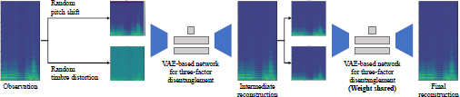
In this paper, we introduce a new re-entry training framework, where the network for three-factor disentanglement is used twice in series (Figure 1). The first network receives the randomly perturbed sound and outputs an intermediate reconstruction. The second network takes it as input and outputs the final reconstruction, with the weights of the two networks being shared. Since the encoders see two different data simultaneously, they are forced to extract sound characteristics that are semantically common to both data. For instance, with respect to pitch, the networks simultaneously process pitch-shifted content (from the perturbed input) and original pitch content (from the intermediate reconstruction), both having the same timbre. As the networks share weights and are thus identical, they are strongly encouraged to focus on extracting semantically consistent features, such as timbre. Additionally, re-entry training implicitly achieves data augmentation because it increases the variety of data that the encoders receive. Moreover, as the training progresses, the intermediate reconstruction gets closer to the original observation, and the encoders of the second network eventually receive almost the same input as the original. This exposes the encoders to a similar situation to the actual inference stage, where the network is used only once and fed inputs without perturbations.
The main contributions of this study are as follows. First, we verify that random pitch shift and timbre distortion play essential roles in achieving the three-factor disentanglement in an unsupervised manner by conducting ablation studies. Second, we formulate a new probabilistic generative model for improved three-factor disentanglement achieved by re-entry training. We theoretically show that the two VAE-based networks in series form a unified large VAE, where the two encoders and the first decoder work as a large inference model, while the second decoder works as a generative model. This allows us to train the entire model still in an unsupervised manner. Third, we quantitatively reveal that the local variational features possess the intended corresponding sound characteristics, such as phoneme information, through experiments with singing voices. Finally, we show that re-entry training can achieve a refined three-factor disentanglement against a wide range of music signals, including those with stationary characteristics (i.e., isolated notes) and with long-lasting non-stationary ones (i.e., monophonic musical fragments or singing voices).
The rest of this paper is organized as follows. Section 2 reviews related work on the disentanglement of music and audio signals. Sections 3 and 4 describe the framework of our previous three-factor disentanglement and those of conventional two-factor disentanglement, respectively. Section 5 explains the re-entry training framework. Section 6 reports comparative experiments, and we develop discussions in Section 7. Section 8 concludes this paper.
2 Related Work
This section reviews existing methods for disentangled representation learning of music signals using autoencoder (AE) or VAE architectures (Sections 2.1 and 2.2). This paper emphasizes an analytical perspective on disentanglement and does not cover differentiable digital signal processing methods [10, 22, 28, 60]. We also explore disentangled representations in speech processing (Section 2.3) and techniques employing weight-shared networks multiple times (Section 2.4) due to their technical similarity to our proposed approach.
2.1 Pitch-conditioned timbre representation learning
Pitch-timbre disentanglement of music signals originated from pitch-conditioned timbre representation learning, primarily utilized in timbre transfer [2, 11, 21]. Early work by Mor et al. [48] introduced AEs for music translation, enabling timbral modifications while preserving pitch. Bitton et al. [4] expanded this approach1 by using the β-VAE model [24] to handle multiple sounds with a single model, allowing many-to-many timbre transfer. Esling et al. [12] proposed a VAE-based method that uses multi-dimensional scaling to align the learned latent timbre space with human perception. Recently, Wu et al. [61] introduced a conditional AE-based model using constant-Q transform representations.
2.2 Pitch-timbre disentanglement
Unconditioned pitch-timbre disentanglement was first explored by Hung et al. [27], who used encoder-decoder structures for music style transfer at the stream level. Recent studies have focused on finer temporal resolutions, such as note-level and frame-level disentanglement. Table 1 summarizes these studies. Techniques vary, including Gaussian mixture VAE [38], unsupervised learning with auxiliary objectives [39], contrastive metric learning [55], two-stage disentangled sequential AEs [41], Jacobian disentangled sequential AEs [42], and random perturbation [54]. However, all aim to disentangle non-stationary music signals into multiple factors with different temporal resolutions. Unlike our previous work [54], this paper addresses non-stationary music signals with various types of music, including isolated notes, monophonic musical fragments, and singing voices.
Comparison of existing works on pitch-timbre disentanglement and the proposed approach.
| Method | Input | Timbre | Pitch | Variation |
|---|---|---|---|---|
| Luo et al. [38] | Spectrogram (stationary) | Global | Global | — |
| Luo et al. [39] | Spectrum | Global | Global | — |
| Tanaka et al. [55] | Spectrogram (stationary) | Local | Local | — |
| Luo et al. [41, 42] | Spectrogram (non-stationary) | Global | Local | — |
| Tanaka et al. [54] (Our previous work) | Spectrogram (stationary) | Global | Local | Local |
| Proposed | Spectrogram (non-stationary) | Global | Local | Local |
2.3 Disentangled representation in speech processing
Disentangled representation learning is also actively explored in speech processing [46, 47], where VAEs have proven effective with vector quantization for unsupervised phoneme extraction [50]. Our approach shares technical similarities with the disentanglement of speech into multiple factors. For instance, Qian et al. [52] decomposed speech signals into rhythms, pitches, timbres, and contents using three information bottlenecks. Similarly, Liu et al. [36] and Liang et al. [34] achieved similar decompositions without requiring bottleneck fine-tuning or hand-crafted features. Choi et al. [7, 8] disentangled speech signals into linguistic, pitch, speaker, and energy information through waveform perturbation, whereas Xie et al. [62] employed a learnable network to extract linguistic information from perturbed speech, contrasting with Choi et al.’s use of a pre-trained wav2vec model. In our research, we align with recent trends in speech processing by applying input signal perturbation with a VAE-based method. However, our research needs to focus on disentangling features unique to music performances, employing tailored perturbation methods.
2.4 Multiple utilization of weight-shared networks
Our proposed re-entry training utilizes weight-shared networks multiple times. This framework has been applied in various audio-related research fields. For example, SpEx+ and SpEx++ [16, 17] employed weight-shared networks in parallel for speaker extraction. Neri et al. [49] used a single VAE twice in parallel to achieve unsupervised blind source separation of musical instrument sounds. Similarly, in the work of Gao and Grauman [14], an audio-visual separator was used in parallel for visually-guided audio source separation, and Wisdom et al. [56, 57] implicitly used the same networks in parallel for unsupervised sound separation. In contrast, Pan et al. [51] used weight-shared networks in series for audio-visual speaker extraction, expecting their progressive refinement architecture to outperform single-stage extraction. Likewise, Hoshen [25] used the same networks in series for image separation. Our method falls into this latter category (i.e., serial use), but differs by integrating two weight-shared networks into a single large VAE, probabilistically formulated in a novel manner.
3 Three-Factor Disentanglement
Our method trains a VAE to disentangle monophonic music signals into global (time-invariant) timbral features and local (time-varying) pitch and variational features in an unsupervised manner (Figure 2). Let x1:N be a matrix consisting of N vectors xn (n = 1,…, N). This VAE is trained to represent the log-amplitude spectrogram X ≜ x1:T ∈ ℝF×T of a monophonic music signal, where F and Τ denote the numbers of frequency bins and time frames, respectively. The proposed training forces the network to estimate the latent representations consisting of global timbres , local variations , and local pitch features from the observations, where D* (* represents “t”, “v”, or “p”) is the dimension of the latent space.
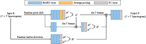
The three-factor VAE model consists of three encoders for inferring latent variables and a decoder for sound generation, ⊕ denotes the concatenation of multiple tensors. During training, the latent variables zt, Zv, and Zp are sampled probabilistically using the reparameterization trick, while during inference, they are given deterministically. Note that random pitch shift and timbre distortion are only applied during training.
The three-factor VAE model consists of three encoders for inferring latent variables and a decoder for sound generation, ⊕ denotes the concatenation of multiple tensors. During training, the latent variables zt, Zv, and Zp are sampled probabilistically using the reparameterization trick, while during inference, they are given deterministically. Note that random pitch shift and timbre distortion are only applied during training.
3.1 Generative, model
We begin by formulating the generative process of an observed log-amplitude spectrogram X. Each time-frequency bin Xfτ ∈ ℝ of X is represented by a Gaussian distribution with latent variables Z,
where is the output of a deep neural network (DNN), decoder with parameters θ, and σ2 ∈ ℝ+ is a hyperparameter representing the variance of the spectrogram. We assume each latent variable follows a standard Gaussian distribution:
where 0D* is the all-zero vector of size D*, and ID* is the identity matrix of size D* × D*. These priors provide each latent variable with independent features [24] that are interpretable.
3.2 Variational inference for unsupervised training
Our goal is to train the DNN to maximize the log-marginal likelihood log pθ (X). However, the DNN-based formulation of our generative model renders log pθ (X) intractable. Instead, we introduce a network, encoder with parameters ϕ, denoted as qϕ(Z|X), to approximate the log-marginal likelihood. We train both the encoder and decoder networks to maximize the following lower bound ℒ of the log-marginal likelihood:
where 𝒟KL(·||·) represents the Kullback-Leibler (KL) divergence. The decoder parameters θ are inferred using maximum likelihood estimation, while the encoder parameters ϕ are optimized to minimize the KL divergence from qϕ(Z|X) to pθ(Z|X) ∝ pθ(X|Z)p(Z). The lower bound can be analytically computed with Monte-Carlo approximation and optimized using gradient ascent.
3.3 DNN-based formulation with partial conditioning
We aim to achieve disentanglement with one global and two local latent features. When these three features are entirely independent, the model may not prioritize the global features or utilize them less due to the dynamic nature of music signals. To compel the model to use the global features, we introduce an inductive bias into its formulation. Specifically, our model needs to disentangle conventional timbre further into global and local features. Therefore, we structure our model so that the global timbral features condition the local variational features while maintaining the independence of pitch features from both.
The formulation of qϕ(Z|X) is now given as
where ϕt, ϕν, and ϕp are the parameters of the encoders for the global timbres, local variations, and local pitch features, respectively. Each posterior is given by
where and are the Dt-dimensional outputs of the DNN with parameters and are the DvT-dimensional outputs with ϕν, and and are the DpT-dimensional outputs with ϕp. The notation [A]τ indicates the τ-th time-frame of A. We approximately calculate the expectation term of ℒ using the reparameterization trick [30] as follows:
where is the reconstructed spectrogram with the samples , and from the variational posterior q. In our model, these samples can be obtained through the following partial ancestral sampling:
3.4 Random perturbation for disentanglement
Our encoders transform the observed spectrogram X into the global timbral representations zt, local variational representations Zv, and local pitch representations Zp. However, these obtained representations are not disentangled in terms of the timbral, variational, and pitch features because all the encoders qϕ* (·) receive the same input feature X, which contains all of the original timbral, variational, and pitch contents. Since the VAE is trained to enable the decoder to reconstruct the observation from the latent features extracted by the encoders, the encoders aim to retain as much information as possible in the latent spaces. Consequently, the timbral, variational, or pitch contents naturally leak into mismatched latent spaces.
To avoid this undesired behavior, we utilize random perturbation techniques. Specifically, we replace the inputs of the encoders X with two types of randomly perturbed spectrograms, and , where “RPS” and “RTD” stand for random pitch shift and timbre distortion (i.e., applying audio effects without changing the pitch), respectively. Let s ≜ s1:L be a time-domain musical signal with a length of L. Originally, the observed spectrogram X is deterministically obtained from the signal s via short-time Fourier transform (STFT) as
Instead, we get the perturbed spectrograms via STFT against randomly perturbed musical signals:
Note that these manipulations modify the signal non-deterministically; the range of pitch shift and the kind of timbre distortion are determined at each attempt.
We can hinder the encoders from extracting undesired information using these perturbed spectrograms. On the one hand, we feed the encoders for the global timbres and local variations with the randomly pitch-shifted spectrograms to prevent them from extracting pitch-related characteristics. On the other hand, we feed the encoder for the local pitch features with the randomly timbre-distorted spectrograms to prevent it from extracting characteristics unrelated to pitch. The formulations of our DNNs (Eqs. (6)-(9)) are thus rewritten as follows:
The ancestral samplings in Eqs. (11)–(13) are also rewritten as follows:
The random pitch shift and timbre distortion of the observed spectrogram make the corresponding representations ignorant of the perturbed aspects of the data. This is because if the randomly perturbed characteristics are extracted by the encoders and used in reconstruction, they deteriorate the likelihood of the model. These perturbations can be introduced without any labels, allowing us to train the VAE in an unsupervised manner. Based on the changes, our VAE is finally trained to maximize the following lower bound ℒR:
Note that the decoder pθ(·) still aims to generate the original observed spectrogram X.
4 Two-Factor Disentanglement
In this paper, we first compare our three-factor disentanglement framework with two kinds of existing two-factor disentanglement frameworks: disentanglement of the global timbres and local pitch features and of the local timbres and local pitch features. This section describes the formulations of these two disentanglement frameworks using random perturbations.
4.1 Disentanglement into global timbre and local pitch
This model is regarded as our model without the local variational features. We aim to estimate the latent representations Z\v ≜ {zt, Zp} from the observation X, where zt and Zp follow a standard Gaussian distribution as described in Eqs. (2) and (4). Each time-frequency bin xfτ∈ ℝ of X is represented with
Similar to Section 3, we approximately calculate the log-marginal likelihood of this model with two encoders and a decoder, where each encoder takes randomly pitch-shifted and timbre-distorted spectrograms as input, respectively:
Each posterior is given by Eqs. (18) and (20), and the samplings (not ancestral) are the same as Eqs. (21) and (23). We train this model to maximize the following lower bound :
4.2 Disentanglement into local timbre and local pitch
This model is then regarded as our model without the global timbral features. Note that the formulation is slightly different from the original one because the local timbres of this model are no longer conditioned. We aim to estimate the latent representations Z\t ≜ {Zv, Zp} from the observation X, where Zv and Zp follow a standard Gaussian distribution as described in Eqs. (3) and (4)2. Each time-frequency bin xfτ∈ ℝ of X is represented with Z\t:
Again, we calculate the log-marginal likelihood of this model. The formulation of the encoders is given as
The first term of the posteriors is derived as
where and are the DvT-dimensional outputs of the DNN with parameters ϕν. The second term is given by Eq. (20). In this model, we obtain the samples independently using
along with Eq. (23). The training of this model is conducted to maximize the following lower bound :
5 Re-entry Training
Our preliminary experiments (Section 6.4) revealed that the three-factor framework explained in Section 3 did not effectively disentangle sounds with pitch transitions or singing voices, causing leakage of local characteristics across different latent features. To address this issue, we introduce a training framework called re-entry training (Figure 3), which employs the network for three-factor disentanglement twice in series with weight sharing.
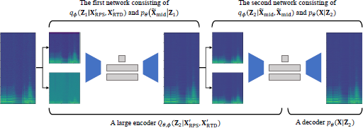
Two interpretations of re-entry training: Serial networks (above representation) can be reinterpreted as a unified large VAE (below representation).
Two interpretations of re-entry training: Serial networks (above representation) can be reinterpreted as a unified large VAE (below representation).
5.1 Re-entry training as two serial networks
In re-entry training, the first network receives the two perturbed inputs and outputs an intermediate reconstruction as follows:
The second network then takes as input for all of its encoders and outputs the final reconstruction X:
The formulations of the components in Eqs. (33)–(36) follow Eqs. (1) and (17)-(23). Re-entry training requires the encoders to simultaneously process two different data: or and , forcing them to focus on specific sound characteristics for extraction. If the encoders capture undesired characteristics from either data, the reconstruction in the other network can be degraded. Specifically, the encoders in the first network are trained to extract as little information as possible, as and are perturbed inputs and likely include unnecessary content. In contrast, the encoders in the second network aim to extract as much information as possible, as is a reconstruction expected to contain only the original content. Since the two networks share weights, excessive filtering by the first network can prevent the second network from fully recovering the lost information, resulting in missing elements and reduced final reconstruction accuracy. Conversely, if the second network retains too much information, it can amplify information leakage in the first network, degrading the intermediate reconstruction quality and, consequently, the final reconstruction accuracy. Additionally, re-entry training doubles the amount of input data received by the encoders, implicitly providing data augmentation and making the network more robust to various data.
5.2 Re-entry training as a unified large VAE
We introduced re-entry training as two serial networks, but it can also be viewed as a unified large VAE, which offers an alternative probabilistic formulation. Specifically, the serial networks can be reinterpreted as a large encoder and a decoder pθ(X|Z2). The formulation of the large encoder is given as follows:
This alternative formulation introduces a nested inference method without altering the original generative model pθ(X|Z2) (i.e., Eq. (1)). It enables us to train the entire model still in an unsupervised manner by maximizing the lower bound ℒRe:
In practice, re-entry training is conducted in parallel with the original VAE training for computational stability, particularly in the early phases, by maximizing the following training objective:
5.3 Inference
Once re-entry training is completed, the latent features can be inferred from unperturbed sounds using Eq. (6) instead of Eq. (17) or Eqs. (37)-(39). On the one hand, as re-entry training progresses, the intermediate reconstruction converges towards the original observation X. Consequently, the encoders of the second network eventually receive inputs that are nearly identical to the original ones, resembling the scenario described in Eq. (6), where unperturbed inputs are fed into the network. On the other hand, as the weights of the encoders qϕ (and the decoder pθ) are shared between the first and second networks, well-trained encoders (i.e., the encoders shown in Eq. (6)) can directly infer disentangled features without utilizing the large encoder. Since the latent variables of a VAE are typically obtained using their means at the inference stage, we can deterministically capture disentangled representations of an input signal.
6 Evaluation
This section reports comparative experiments conducted to evaluate the effectiveness of re-entry training. We first assessed the three-factor disentanglement framework against the two conventional two-factor frameworks, highlighting its limitations, particularly in handling singing voices (Section 6.4). Subsequently, we compared the standard three-factor method with re-entry training, showing that re-entry training achieved more refined disentanglement than the standard method across various music signals, including isolated notes, monophonic musical fragments, and singing voices (Sections 6.5 and 6.6). Also, we conducted ablation studies to examine the contributions of the random pitch shift and timbre distortion in our unsupervised training scheme, as well as the effects of batch size on singing voices and the choice of k in the k-nearest neighbor classifiers used for evaluation (Section 6.7).
6.1 Data
Through our experiments, we used the following three types of music signals from different datasets.
Isolated notes. We used isolated notes from a subset of the RWC Music Database [18]. Each file is annotated with the instrument name and spans the entire pitch range of the instrument at semitone intervals. We segmented each file into isolated notes using silence detection and removed initial silent sections identified by onset detection. From the initial 88,889 files, we selected 62,704 files covering pitches from A0 to C8 (excluding percussive instruments), corresponding to 43 distinct instrument classes. For evaluation, we randomly split the pitched sounds into three sets: a training set (43,892 files), a validation set (9,406 files), and a test set (9,406 files). Only the first two seconds of each sound were used for analysis. The resulting spectrograms had dimensions F = 2049 and T ≤ 201.
Monophonic musical fragments. We used monophonic musical fragments from the Slakh2100-redux dataset [44], consisting of 1,289 training tracks, 270 validation tracks, and 151 test tracks. Each track includes isolated, synthesized audio for multiple instruments along with accompanying MIDI data. The dataset spans 83 distinct instrument classes, including a wide variety of synthesized timbres. To extract monophonic segments, we filtered out polyphonic segments longer than 100 ms and silent segments longer than two seconds based on the MIDI data. Segments longer than three seconds were considered valid and randomly trimmed to a maximum of five seconds. The resulting spectrograms had dimensions F = 2049 and T ≤ 501. Instrument names were identified using the General MIDI program numbers, excluding drums.
Singing voices. We used singing voice recordings from the PJS dataset [31], which includes 100 phoneme-balanced short songs (totaling 27.2 minutes) sung by a Japanese male singer. Each song is annotated with MIDI data and temporally aligned phoneme labels. For evaluation, we randomly split the songs into a training set (70 files), a validation set (15 files), and a test set (15 files). The songs were randomly cut into five-second segments, and the resulting spectrograms had dimensions F = 2049 and T = 501.
All sounds were sampled at 44.1 kHz. During training, we applied random pitch shifts and timbre distortions to each sound on the fly. Specifically, the pitch was shifted by L semitones (−7 ≤ L ≤ 7), with L chosen from a uniform distribution (including L = 0) for each instance. Timbre distortion was applied using Pedalboard3, a Python library by Spotify. Two out of nine presets (Chorus, Distortion, Phaser, LadderFilter, HighpassFilter, LowpassFilter, Reverb, GSMFullRateCompressor, and Bitcrush) were randomly selected and applied to the sound each time. We used STFT with a Hann window of 4,096 samples and a hop size of 441 samples (10 ms). The spectrograms were normalized to have an average amplitude of one. Our implementation utilized the librosa library [45].
6.2 Model configuration
Our VAE utilizes the bidirectional gated recurrent unit (BiGRU) architecture for its encoders and decoder to capture the temporal characteristics of sounds, as shown in Figure 2. All the BiGRU layers have 2 × 800 cells. First, the randomly pitch-shifted sounds are fed into the encoder for the global timbres and the encoder for the local variations. The encoder for the global timbres consists of three BiGRU layers, an average pooling layer along the time-frame axis, and fully connected (FC) layers. Two FC layers independently transform the 1,600-dimensional output into Dt dimensions to represent the means and variances of the latent variables. The encoder for the local variations also consists of three BiGRU layers and FC layers. The global timbres are tiled along the time-frame axis and fed into the last BiGRU layer concatenated with the outputs of the second BiGRU layer along the spatial axis (i.e., the final BiGRU layer takes input tensors with (Dt + 1, 600) dimensions). Two FC layers perform the same transformation as those for the global timbres.
Next, the randomly timbre-distorted sounds are fed into the encoder for the local pitch features. This encoder consists of three BiGRU layers and FC layers. These FC layers independently transform the 1,600-dimensional output into Dp dimensions to represent the means and variances of the latent variables. Finally, the decoder reconstructs the observation from the three types of latent variables above. Note that these variables are sampled probabilistically during training but are given deterministically during inference using their means. The decoder consists of three BiGRU layers and an FC layer. The tiled global timbral, local variational, and local pitch features are all concatenated along the spatial axis and fed into the decoder (i.e., the first BiGRU layer takes input tensors with (Dt + Dv + Dp) dimensions). The final FC layer transforms the 1,600-dimensional output into the same dimensions as the observation, F. The three FC layers representing the variances of the latent variables are passed through the softplus activation function. We set σ2 in Eq. (1) to 0.5.
The dimensions Dt, Dv, and Dp were experimentally set to 64, 64, and 32, respectively. In the experiments with isolated notes from RWC and monophonic musical fragments from Slakh2100-redux, the batch size was set to 32. In the experiments with singing voices from PJS, the batch size was set to one. We used the Adam optimizer [29] with an initial learning rate of 1.0 × 10⁻⁴ for RWC and Slakh2100-redux and 1.0 × 10⁻⁵ for PJS. The learning rate was reduced exponentially by 0.01% per epoch. We applied cyclical annealing of KL regularization [13] from zero to one every ten epochs. The checkpoints that achieved the best validation loss were used for the final evaluations.
6.3 Evaluation criteria
We evaluated the degree of disentanglement in each latent space by calculating the accuracy of instrument classification and pitch estimation for isolated notes and monophonic musical fragments, as well as phoneme estimation and pitch estimation for singing voices. If the latent spaces are ideally disentangled, each of the latent features, such as the pitch feature, should not contain information about other characteristics, such as timbral or variational characteristics. To assess this, we used k-nearest neighbor (k-NN) classifiers. For isolated notes and monophonic musical fragments, we used their training sets with instrument names and semitone-level pitch annotations. For singing voices, we employed phoneme labels and semitone-level pitch annotations. Note that we excluded the silent segments here.
We chose k-NN classifiers because they can directly capture the structure of each latent space with sufficient accuracy without requiring additional model development and parameter tuning, unlike DNN-based methods. The accuracy should be high exclusively within the corresponding space. Note that the construction of the k-NN classifier is performed sample-wise for the global features and frame-wise for the local features. Therefore, for the global features, each vote is based on an individual input sample, while for the local features, each vote is based on an individual frame within the input sample4. Throughout our experiments, we set k to 5.
We also assessed the quality of spectrogram reconstruction to monitor potential information loss through disentangled representations. We computed the mean squared error (MSE) between the input log-amplitude spectrogram X and the output log-amplitude spectrogram per time-frequency bin on the test data. As we employed the deep generative model formulation in Eq. (1) with a fixed σ2 = 0.5, the MSE corresponds to the negative log-likelihood for X, with a lower MSE indicating better reconstruction quality.
6.4 Preliminary experiments
We first compared the three-factor disentanglement framework with the two-factor frameworks, demonstrating its advantages and limitations.
6.4.1 Isolated notes
The three-factor framework demonstrated superior disentanglement performance on isolated notes, as indicated by the comparative evaluations of two-factor and three-factor disentanglement methods in Table 2. The global timbral features were crucial for extracting instrument information, achieving classification accuracies exceeding 90% for both methods. In contrast, the accuracy using the local variational features was below 80%. Note that “Variation” in the table (and the following tables) has arrows in different directions for different systems. This is because it represents the local timbres in the two-factor method and the local variational features in the three-factor method (also see Section 4.2). The performance gap between the global timbral features of the two-factor method (97.6%) and the three-factor method (94.7%) was around 3%.
For pitch estimation, incorporating local variational features improved the performance of the local pitch features. Specifically, the pitch-timbre disentanglement method scored below 40%, whereas the other methods achieved above 50%, with the three-factor method showing the highest performance. As such, the gain in pitch estimation accuracy was significantly greater than the loss in instrument classification accuracy (3%). This suggests that the local variational features effectively capture the time-variant characteristics of isolated notes unrelated to pitch, thereby refining the disentanglement of the local pitch features. Moreover, richer features contribute to minimizing information loss through disentangled representations, as evidenced by the MSE scores (0.609 > 0.557 > 0.543).
Comparison of the two-factor and three-factor disentanglement on isolated notes. In this and the following tables, ↑ indicates that higher values are better, while ↓ indicates that lower values are better.
| Factors | MSE ↓ | Instrument classification [%] | Pitch estimation [%] | ||||||
|---|---|---|---|---|---|---|---|---|---|
| Timbre | Variation | Pitch | Timbre ↑ | Variation | Pitch ↓ | Timbre ↓ | Variation ↓ | Pitch ↑ | |
| ✓ | ✓ | 0.609 | 97.6 | — | 31.8 | 7.8 | — | 34.5 | |
| ✓ | ✓ | 0.557 | — | 77.5 (↑) | 37.4 | — | 13.2 | 51.9 | |
| ✓ | ✓ | ✓ | 0.543 | 94.7 | 54.6 (↓) | 38.5 | 15.8 | 7.0 | 61.6 |
6.4.2 Monophonic musical fragments
Table 3 presents comparative evaluations of monophonic musical fragments, indicating the three-factor framework generally achieved superior disentanglement. Note that the instrument classification task in this dataset is particularly challenging due to the larger number of instrument classes compared to isolated notes. Additionally, instruments with similar timbres (e.g., acoustic grand piano and bright acoustic piano, treated as separate classes) further increase the complexity of classification. Similar to isolated notes, the global timbral features proved more effective than the local variational features in extracting instrument information. However, examining the accuracy gaps among the three features within the three-factor method revealed much smaller discrepancies (51.2% − 37.3% − 30.0%) compared to the more significant differences observed in isolated notes (94.7% − 54.6% − 38.5%). Ideally, these differences should be substantial, as seen in the isolated notes, but that was not the case here. This suggests that while the three-factor method outperformed the two-factor methods, the disentanglement remained less effective for monophonic musical fragments.
Comparison of two-factor and three-factor disentanglement on monophonic musical fragments.
| Factors | MSE ↓ | Instrument classification [%] | Pitch estimation [%] | ||||||
|---|---|---|---|---|---|---|---|---|---|
| Timbre | Variation | Pitch | Timbre ↑ | Variation | Pitch ↓ | (Timbre ↓) | Variation ↓ | Pitch ↑ | |
| ✓ | ✓ | 0.524 | 47.1 | — | 31.6 | (N/A) | — | 69.3 | |
| ✓ | ✓ | 0.452 | — | 44.4 (↑) | 35.7 | (—) | 37.2 | 77.8 | |
| ✓ | ✓ | ✓ | 0.446 | 51.2 | 37.3 (↓) | 30.0 | (N/A) | 27.7 | 74.9 |
Regarding pitch estimation, it is no longer possible to infer any pitch information from the global timbral features due to the time-variant characteristics of pitch transitions; thus, this is marked as N/A. The local pitch features of all three methods were comparable in terms of pitch estimation accuracy. However, the three-factor method showed a reduced accuracy with the local variational features (27.7%), indicating a higher degree of disentanglement than the two-factor method. Similar to the results with isolated notes, having more latent features led to less information loss, as evidenced by the MSE scores. Notably, the absence of local variational features had a significantly negative impact on MSE.
6.4.3 Singing voices
Table 4 shows comparative evaluations of singing voices, indicating that both the two-factor and three-factor disentanglement frameworks did not achieve effective disentanglement. Note that the global timbral features were not applicable, as phonemes and pitch transitions are time-variant characteristics, hence marked as N/A. First, the pitch-timbre disentanglement method resulted in outcomes opposite to the ideal. The performance of phoneme estimation using its local pitch features (64.7%) was far higher than that of pitch estimation (16.6%). The other two methods also resulted in inadequate performance. They extracted the pitch characteristics of singing voices to some extent using the local pitch features. However, the variational characteristics (i.e., phoneme information) were also contaminated in the features, resulting in small performance gaps for phoneme estimation between the two local features (62.1% vs 46.3% and 61.4% vs 48.1%). Incidentally, the MSE scores were overall worse than those in the other two datasets. This is likely due to the size of the PJS dataset; only 70 songs were available for training.
Comparison of two-factor and three-factor disentanglement on singing voices.
| Factors | MSE ↓ | Phoneme estimation [%] | Pitch estimation [%] | ||||||
|---|---|---|---|---|---|---|---|---|---|
| Timbre | Variation | Pitch | (Timbre ↓) | Variation ↑ | Pitch ↓ | (Timbre ↓) | Variation ↓ | Pitch ↑ | |
| ✓ | ✓ | 0.873 | (N/A) | — | 64.7 | (N/A) | — | 16.6 | |
| ✓ | ✓ | 0.653 | (—) | 62.1 | 46.3 | (—) | 13.3 | 44.2 | |
| ✓ | ✓ | ✓ | 0.613 | (N/A) | 61.4 | 48.1 | (N/A) | 12.7 | 45.5 |
To further investigate this aspect, we examined whether a performance gap exists across different split sets. The results are presented in Table 5. For the training data, we randomly split the 70 samples into 56 for constructing k-NN classifiers and 14 for assessment. The results show minimal performance differences between the various splits, indicating that the training process was conducted properly. However, the relatively small number of training samples appears insufficient for the three models to effectively learn disentangled representations.
Performance of two-factor and three-factor disentanglement on singing voices across different split sets.
| Data split | Factors | MSE ↓ | Phoneme estimation [%] | Pitch estimation [%] | ||||
|---|---|---|---|---|---|---|---|---|
| Timbre | Variation | Pitch | Variation ↑ | Pitch ↓ | Variation ↓ | Pitch ↑ | ||
| Test | ✓ | ✓ | 0.873 | — | 64.7 | — | 16.6 | |
| Test | ✓ | ✓ | 0.653 | 62.1 | 46.3 | 13.3 | 44.2 | |
| Test | ✓ | ✓ | ✓ | 0.613 | 61.4 | 48.1 | 12.7 | 45.5 |
| Training | ✓ | ✓ | 0.897 | — | 63.8 | — | 14.9 | |
| Training | ✓ | ✓ | 0.650 | 62.4 | 44.4 | 11.5 | 43.0 | |
| Training | ✓ | ✓ | ✓ | 0.605 | 61.5 | 44.2 | 10.7 | 45.2 |
| Validation | ✓ | ✓ | 0.888 | — | 63.2 | — | 17.8 | |
| Validation | ✓ | ✓ | 0.657 | 60.9 | 44.0 | 12.8 | 45.0 | |
| Validation | ✓ | ✓ | ✓ | 0.614 | 60.3 | 46.2 | 11.1 | 47.3 |
Throughout all the preliminary experiments, the three-factor disentanglement method outperformed the two-factor methods, yet it remained inadequate as a general disentangled representation for various monophonic music signals.
6.5 Performance of re-entry training
We compared the standard three-factor disentanglement method with re-entry training framework. Hereafter, we refer to the former as the standard method. We also evaluated re-entry training against three baselines to assess its benefits, specifically its ability to implicitly provide data augmentation and simulate the inference phase by incorporating unperturbed inputs during training. For the baselines, we implemented simple data augmentation by adding random noise (i.e., white noise) to the original samples and introduced a 25% perturbation dropout to feed unperturbed inputs during training in the standard method.
6.5.1 Isolated notes
Table 6 presents the results on isolated notes. Compared to the standard method, re-entry training generally reduced the accuracies of both instrument classification and pitch estimation across all features, accompanied by a deterioration in the MSE score. Although the introduction of re-entry training did not significantly impact the results for this type of music signal, a notable aspect is that it did not impede the training processes of the three-factor disentanglement. Despite a decrease in pitch estimation scores on the local pitch features, all features maintained a high level of disentanglement.
The standard methods with random noise achieved the highest pitch estimation accuracies on the local pitch features. However, the sound characteristics were more evenly distributed across the three features, leading to smaller performance discrepancies, especially in instrument classification accuracy. When combined with perturbation dropout alone, MSE and instrument classification scores surpassed those of re-entry training, but the pitch estimation accuracy gap between the global timbral and local pitch features narrowed significantly. The results are also observed to be more strongly affected by random noise than by perturbation dropout when both are applied. These results suggest that re-entry training effectively combines the benefits of the baselines, i.e., data augmentation and inference-phase simulation.
Comparison of the standard three-factor disentanglement methods with re-entry training framework on isolated notes. In this and subsequent tables, RN and PD refer to adding random noise and introducing perturbation dropout, respectively.
| Methods | MSE ↓ | Instrument classification [%] | Pitch estimation [%] | ||||
|---|---|---|---|---|---|---|---|
| Timbre ↑ | Variation ↓ | Pitch ↓ | Timbre ↓ | Variation ↓ | Pitch ↑ | ||
| Standard | 0.543 | 94.7 | 54.6 | 38.5 | 15.8 | 7.0 | 61.6 |
| Standard + RN | 0.697 | 91.6 | 67.7 | 63.5 | 15.2 | 8.7 | 79.0 |
| Standard + PD | 0.536 | 95.9 | 44.5 | 35.1 | 24.7 | 5.0 | 47.1 |
| Standard + RN + PD | 0.666 | 94.4 | 71.4 | 73.4 | 12.8 | 9.2 | 80.6 |
| Re-entry | 0.594 | 92.1 | 52.7 | 37.0 | 9.8 | 5.1 | 49.2 |
6.5.2 Monophonic musical fragments
Table 7 presents the results on monophonic musical fragments, illustrating that re-entry training improved the quality of disentanglement compared to the standard method. For instrument classification accuracy, while the score moderately increased with the local pitch features (from 30.0% to 37.5%), it significantly decreased with the local variational features (from 37.3% to 19.3%) without impacting the score with the global timbral features. These findings indicate that re-entry training mitigated the small discrepancies observed in the standard method. In terms of pitch estimation, re-entry training notably enhanced disentanglement. Specifically, the accuracy with the local variational features decreased significantly from 27.7% with the standard method to 11.1% with re-entry training. Conversely, the accuracy with the local pitch features increased from 74.9% to 79.3%, resulting in a wider performance gap.
Comparison of the standard three-factor disentanglement methods with re-entry training framework on monophonic musical fragments.
| Methods | MSE ↓ | Instrument classification [%] | Pitch estimation [%] | ||||
|---|---|---|---|---|---|---|---|
| Timbre ↑ | Variation ↓ | Pitch ↓ | (Timbre ↓) | Variation ↓ | Pitch ↑ | ||
| Standard | 0.446 | 51.2 | 37.3 | 30.0 | (N/A) | 27.7 | 74.9 |
| Standard + RN | 0.814 | 23.5 | 31.0 | 43.4 | (N/A) | 13.6 | 80.2 |
| Standard + PD | 0.440 | 44.3 | 32.5 | 42.3 | (N/A) | 17.7 | 82.3 |
| Standard + RN + PD | 0.862 | 39.5 | 28.2 | 45.4 | (N/A) | 10.0 | 82.5 |
| Re-entry | 0.431 | 51.2 | 19.3 | 37.5 | (N/A) | 11.1 | 79.3 |
A noteworthy observation in this dataset is the substantial accuracy decrease when using the local variational features with re-entry training. This suggests that the model under the standard method did not effectively distinguish the two local features, leading to undesired characteristics bleeding into other features. Additionally, it is important to highlight that the MSE score improved from 0.446 to 0.431, indicating a more focused extraction of sound characteristics for enhanced reconstruction quality, as anticipated.
The three baseline methods yielded notable findings for instrument classification. While adding random noise and introducing perturbation dropout degraded accuracies on the global timbral and local pitch features, these negative effects were mitigated with re-entry training. Conversely, both methods improved accuracies on the local variational features, and these improvements were amplified when combined with re-entry training. These results indicate that re-entry training effectively integrates the benefits of data augmentation and inference-phase simulation, mirroring the trends observed in the case of isolated notes.
6.5.3 Singing voices
Table 8 presents the results on singing voices, showing mixed results with re-entry training. Regarding phoneme estimation accuracy, while the score with the local variational features remained nearly the same compared to the standard method (61.4% vs 60.7%), the score with the local pitch features significantly decreased from 48.1% to 33.9%. This result indicates that re-entry training improved the quality of the local pitch features by eliminating the contamination of local variational characteristics of sounds. However, for pitch estimation accuracy, the scores with both the local variational and pitch features decreased, with the drop in pitch features being more substantial. This implies that while re-entry training helps eliminate contamination, it may also inadvertently remove essential information.
Comparison of the standard three-factor disentanglement methods with re-entry training framework on singing voices.
| Methods | MSE ↓ | Phoneme estimation [%] | Pitch estimation [%] | ||||
|---|---|---|---|---|---|---|---|
| (Timbre ↓) | Variation ↑ | Pitch ↓ | (Timbre ↓) | Variation ↓ | Pitch ↑ | ||
| Standard | 0.613 | (N/A) | 61.4 | 48.1 | (N/A) | 12.7 | 45.5 |
| Standard + RN | 1.130 | (N/A) | 60.8 | 58.5 | (N/A) | 11.9 | 53.2 |
| Standard + PD | 0.594 | (N/A) | 60.9 | 44.8 | (N/A) | 12.5 | 44.0 |
| Standard + RN + PD | 1.110 | (N/A) | 60.7 | 58.2 | (N/A) | 11.7 | 51.1 |
| Re-entry | 0.590 | (N/A) | 60.7 | 33.9 | (N/A) | 10.9 | 33.6 |
Additionally, re-entry training successfully reduced the MSE score from 0.613 to 0.590. Given that the total amount of extracted latent information decreased, as mentioned above, this suggests that the focused extraction of sound characteristics also improved reconstruction quality for singing voices, echoing similar results observed in monophonic musical fragments. Interestingly, the improvement in the MSE score was most pronounced among the three types of music signals. This is likely due to the stronger effect of implicit data augmentation, considering the PJS dataset comprises only 100 songs in total, whereas Slakh2100-redux contains 1,710 tracks with much longer durations. Although merely augmenting data (e.g., by adding random noise) may worsen the MSE scores, it appears to work promisingly across the three datasets when combined with the inference-phase simulation in re-entry training. Furthermore, directly incorporating data augmentation or unperturbed samples tends to produce extreme results, while utilizing both through re-entry training leads to more balanced performance.
Through all the comparative experiments between the standard method and re-entry training framework, the model with re-entry training demonstrated an ability to acquire more focused latent information. This effect was notable and introduced some trade-offs: while it helped eliminate unnecessary information, thereby enhancing the quality of each latent feature, it also risked excluding essential information. Generally, re-entry training refined (i.e., widened) the performance gap among the three features by improving the quality of the local variational features, though this came at the cost of some desired information in the local pitch features.
6.6 Comparison of encoder types in re-entry training
As outlined in Section 5.3, once re-entry training is completed, disentangled representations can be inferred using the small encoder (i.e., Eq. (6)), rather than the large encoder (i.e., Eqs. (37)-(39)). However, it remains essential to assess how the choice between these two encoder types affects the disentangled representations and reconstruction performance. Comparative results are provided in Tables 9, 10, and 11, with the decoder being consistently defined as Eq. (1).
Comparison of two types of latent representations obtained using small and large encoders during re-entry training on isolated notes.
| Encoder | MSE ↓ | Instrument classification [%] | Pitch estimation [%] | ||||
|---|---|---|---|---|---|---|---|
| Timbre ↑ | Variation ↓ | Pitch ↓ | Timbre ↓ | Variation ↓ | Pitch ↑ | ||
| Small | 0.594 | 92.1 | 52.7 | 37.0 | 9.8 | 5.1 | 49.2 |
| Large | 0.612 | 93.3 | 66.1 | 53.1 | 11.8 | 8.9 | 60.8 |
In general, the disentangled representations obtained with the small encoder outperformed those derived from the large encoder in terms of both potential information loss and disentanglement quality. Specifically, all three MSE scores deteriorated when the large encoder was used, and the values measured across the three latent features increased. This outcome is expected for the large encoder, as its multi-stage processes introduce cumulative information loss. Consequently, intermediate reconstructions tend to lose distinctive characteristics and become smoothed across samples, resulting in less effective disentanglement and higher error metrics.
Comparison of two types of latent representations obtained using small and large encoders during re-entry training on monophonic musical fragments.
| Encoder | MSE ↓ | Instrument classification [%] | Pitch estimation [%] | ||||
|---|---|---|---|---|---|---|---|
| Timbre ↑ | Variation ↓ | Pitch ↓ | (Timbre ↓) | Variation ↓ | Pitch ↑ | ||
| Small | 0.431 | 51.2 | 19.3 | 37.5 | (N/A) | 11.1 | 79.3 |
| Large | 0.443 | 51.8 | 30.7 | 40.5 | (N/A) | 23.9 | 82.0 |
Comparison of two types of latent representations obtained using small and large encoders during re-entry training on singing voices.
| Encoder | MSE ↓ | Phoneme estimation [%] | Pitch estimation [%] | ||||
|---|---|---|---|---|---|---|---|
| (Timbre ↓) | Variation ↑ | Pitch ↓ | (Timbre ↓) | Variation ↓ | Pitch ↑ | ||
| Small | 0.590 | (N/A) | 60.7 | 33.9 | (N/A) | 10.9 | 33.6 |
| Large | 0.634 | (N/A) | 62.0 | 40.6 | (N/A) | 12.1 | 37.3 |
When comparing the large encoder results to the standard method reported in Tables 2, 3, and 4, the performance degraded for isolated notes but showed some improvement for monophonic musical fragments and singing voices. This suggests that while the large encoder may excel at handling complex or continuous input patterns, its overall effectiveness is constrained for data with simpler characteristics.
6.7 Ablation study
We examined the contributions of the random pitch shift and timbre distortion in our unsupervised training scheme. We also assessed the impacts of batch size on singing voices and k selection in the k-NN.
6.7.1 Contributions of random pitch shift and timbre distortion
We further investigated the contributions of random pitch shift and timbre distortion to achieving three-factor disentanglement in an unsupervised manner. To assess their impact, we conducted experiments where either or both random perturbations were removed during the standard training. We evaluated performance across the three types of music signals. The results are detailed in Tables 12, 13, and 14.
Effect of random perturbations on disentanglement in isolated notes.
| Perturbations | MSE ↓ | Instrument classification [%] | Pitch estimation [%] | |||||
|---|---|---|---|---|---|---|---|---|
| RPS | RTD | Timbre ↑ | Variation ↓ | Pitch ↓ | Timbre ↓ | Variation ↓ | Pitch ↑ | |
| 0.438 | 96.8 | 13.0 | 21.5 | 90.8 | 8.2 | 12.5 | ||
| ✓ | 0.475 | 97.3 | 20.9 | 39.2 | 11.8 | 4.0 | 28.1 | |
| ✓ | 0.473 | 97.5 | 17.4 | 42.6 | 84.9 | 5.8 | 13.5 | |
| ✓ | ✓ | 0.543 | 94.7 | 54.6 | 38.5 | 15.8 | 7.0 | 61.6 |
Effect of random perturbations on disentanglement in monophonic musical fragments.
| Perturbations | MSE ↓ | Instrument classification [%] | Pitch estimation [%] | |||||
|---|---|---|---|---|---|---|---|---|
| RPS | RTD | Timbre ↑ | Variation ↓ | Pitch ↓ | (Timbre ↓) | Variation ↓ | Pitch ↑ | |
| 0.414 | 53.6 | 40.4 | 12.2 | (N/A) | 76.8 | 17.4 | ||
| ✓ | 0.439 | 20.6 | 34.2 | 44.1 | (N/A) | 23.8 | 78.6 | |
| ✓ | 0.448 | 53.4 | 18.8 | 26.8 | (N/A) | 12.3 | 72.0 | |
| ✓ | ✓ | 0.446 | 51.2 | 37.3 | 30.0 | (N/A) | 27.7 | 74.9 |
Effect of random perturbations on disentanglement in singing voices.
| Perturbations | MSE ↓ | Phoneme estimation [%] | Pitch estimation [%] | |||||
| RPS | RTD | (Timbre ↓) | Variation ↑ | Pitch ↓ | (Timbre ↓) | Variation ↓ | Pitch ↑ | |
| 0.524 | (N/A) | 39.8 | 45.9 | (N/A) | 39.5 | 36.1 | ||
| ✓ | 0.562 | (N/A) | 61.4 | 55.7 | (N/A) | 16.0 | 39.1 | |
| ✓ | 0.557 | (N/A) | 57.5 | 34.9 | (N/A) | 30.4 | 55.8 | |
| ✓ | ✓ | 0.613 | (N/A) | 61.4 | 48.1 | (N/A) | 12.7 | 45.5 |
First, we examined the outcomes when random pitch shift was omitted. The absence of this perturbation noticeably deteriorated disentanglement within the global timbral and local variational features. As shown in Table 12, pitch information of isolated notes leaked into the global timbral features, resulting in significantly higher pitch estimation accuracies than the local pitch features. Table 14 also indicates decreased phoneme estimation accuracy when using the local variational features. Furthermore, pitch estimation accuracies generally decreased when using the local pitch features, except in cases involving singing voices with random timbre distortion (Tables 12, 13, and 14). These results emphasize the critical role of random pitch shift in achieving effective three-factor disentanglement.
Next, we analyzed the results when random timbre distortion was omitted. The absence of this perturbation led to an overall deterioration in disentanglement within the local pitch features. Tables 12, 13, and 14 illustrate decreased pitch estimation accuracies using the local pitch features under various conditions, except for singing voices with random pitch shift. Table 14 also reveals that variational information from singing voices leaked into the local pitch features, resulting in phoneme estimation accuracies comparable to or even higher than those using the local variational features. This phenomenon also had a detrimental effect on the local variational features. These results indicate the importance of random timbre distortion in our method.
Finally, it is important to note that both random perturbations degraded the quality of spectrogram reconstruction. Across all ablation studies, introducing an additional perturbation consistently worsened reconstruction quality. Applying both perturbations simultaneously had an even more detrimental effect compared to using either one alone. This result was anticipated beforehand, as the concurrent application of both perturbations hindered our VAE from learning from the original input during training.
6.7.2 Impact of batch size on singing voices
Since the singing voice dataset is considerably smaller than the other two datasets, we set the batch size for this dataset to one, while using a batch size of 32 for the other datasets. This discrepancy in batch sizes may have contributed to the performance gap, particularly the poorer performance observed for the singing voices. To further investigate this, we conducted re-entry training experiments on the singing voice dataset with batch sizes varying up to 32. The results presented in Table 15 indicate that larger batch sizes resulted in less effective training, with trends deviating from the expected behavior. Specifically, larger batch sizes resulted in higher MSE scores, lower phoneme estimation scores on the local variational features, and higher scores on the local pitch features. Although the pitch estimation scores on the local variational features slightly improved, those on the local pitch features worsened. These findings support our decision to use a batch size of one for the singing voice dataset.
Performace of re-entry training on singing voices with different batch sizes.
| Batch size | MSE ↓ | Phoneme estimation [%] | Pitch estimation [%] | ||||
|---|---|---|---|---|---|---|---|
| (Timbre ↓) | Variation ↑ | Pitch ↓ | (Timbre ↓) | Variation ↓ | Pitch ↑ | ||
| 1 | 0.590 | (N/A) | 60.7 | 33.9 | (N/A) | 10.9 | 33.6 |
| 4 | 0.635 | (N/A) | 60.6 | 43.5 | (N/A) | 11.2 | 31.1 |
| 8 | 0.700 | (N/A) | 60.6 | 49.0 | (N/A) | 9.9 | 24.2 |
| 16 | 0.776 | (N/A) | 58.6 | 53.7 | (N/A) | 8.8 | 13.1 |
| 32 | 0.875 | (N/A) | 52.8 | 55.3 | (N/A) | 8.3 | 11.5 |
6.7.3 Impact of k choice in the k-NN classifier
As noted in Section 6.3, we consistently set k to 5 in the k-NN classifier throughout all experiments. However, the frame-wise voting method could introduce noise due to this choice of k. To further explore this, we conducted additional experiments focusing on instrument classification on the local variational features. The results, summarized in Table 16, show that the scores remain largely unchanged across different k values. This finding also supports our decision to set k to 5.
7 Discussion
Our proposed three-factor disentanglement framework achieved better results than the conventional two-factor frameworks and was more successful with re-entry training. However, there are two main drawbacks regarding the perturbations. First, while the random pitch shift can effectively eliminate target characteristics (i.e., pitch information) from input sounds, the random timbre distortion used in this study cannot achieve the same effect. This is because the distortions introduced in Section 6.1 are designed to add audio effects to an instrument while preserving its instrumental identity. Consequently, timbral characteristics can leak into the local pitch features, as observed in our preliminary experiments on singing voices. Although re-entry training alleviated this issue, further disentanglement is desired. One solution might be to replace the timbre distortion with DNN-based timbre transfer networks instead of traditional signal processing techniques. However, this would require labels and semi- or fully supervised training.
Second, there is also potential for improvement in mitigating the side effects caused by the perturbations. As observed in the ablation studies, the perturbations are essential for unsupervised three-factor disentanglement but also degrade the quality of spectrogram reconstruction. This means that the overall model performance diminishes from the perspective of a generative model. It is important to note that our focus was on the framework-level method rather than DNN architectures, which is why we used relatively simple DNNs, such as BiGRUs. Since the re-entry training framework can be integrated with other architectures, this issue can be addressed by employing more expressive DNNs (e.g., transformers) for the decoder.
We focused on pitched instruments in this paper, but another vital family of instruments used in music is percussive instruments. Treating them within the same disentanglement framework as pitched instruments is challenging yet interesting. In fact, the proposed method failed to achieve this, with all three latent features having similar representations and attaining almost the same accuracies in any evaluations (these experiments were conducted as trials and are not reported in this paper). This is not surprising because our method used the random “pitch” shift, which cannot be well-defined for percussive instruments. To address this, we need to reconsider how musical sounds should be interpreted and disentangled.
In addition, the trained models are currently tailored to each specific dataset. From a generalizability perspective, it is worth investigating the creation of a model capable of handling musical sounds from multiple datasets. Ultimately, a method for disentangling polyphonic music signals that can simultaneously manage multiple musical sounds is desirable. This advancement would pave the way for future applications, including zero-shot automatic music transcription.
8 Conclusion
In this paper, we presented the re-entry training framework to enhance pitch-timbre-variation disentanglement of monophonic music signals based on random perturbation. This framework applied the network for three-factor disentanglement twice in series with weight sharing, refining the characteristics extracted by the encoders and implicitly achieving data augmentation. The serial model was trained in an unsupervised manner, leveraging its alternative probabilistic formulation as a unified large VAE. Our experiments demonstrated that reentry training achieved effective disentanglement across a wide range of music signals, including isolated notes, monophonic musical fragments, and singing voices. Additionally, we confirmed the necessity of two types of random perturbation on input sounds for successful disentanglement within our framework. Looking ahead, we aim to extend our method to handle polyphonic music signals and percussive instruments, further broadening the applicability and robustness of our disentanglement framework.
The paper by Mor et al. [48] was accepted to ICLR in 2019 but was submitted to arXiv on 21 May 2018 (https://arxiv.org/abs/1805.07848). Meanwhile, the paper by Bitton et al. [4] was submitted to arXiv on 29 September 2018.
Naturally, the local timbres of this model should be denoted as . However, this usage clashes with zt (i.e., the global timbres) and confuses correspondence to the three-factor model, hence Zv.
Particularly for instrument classification on the local variational features, an alternative approach is to average the latent features across time and classify based on the averaged vector. In this study, as our focus is on comparing the frameworks, we opted for the frame-wise method without averaging, as it better captures the diversity of features at each frame. However, the aspect of temporal granularity and information capacity remains an important topic of discussion [33, 37, 40, 41].
This work is supported by Frontier of Embodiment Informatics: ICT and Robotics, under Waseda University’s Waseda Goes Global Plan, as part of The Japanese Ministry of Education, Culture, Sports, Science and Technology (MEXT)’s Top Global University Project. This work is also supported by JSPS KAKENHI Nos. 22KJ2959, 24H00742, 24H00748, JST PRESTO No. JPMJPR20CB, and JST FOREST No. JPMJFR2270.
