


Extensive evaluation on a large number of word embedding models for language processing applications is conducted in this work. First, we introducepopularword embeddingmodelsanddiscussdesiredproperties of wordmodels andevaluationmethods (or evaluators). Then, we categorize evaluators into intrinsic and extrinsic two types. Intrinsic evaluators test the quality of a representation independent of specific natural language processing tasks while extrinsic evaluators use word embeddings as input features to a downstream task and measure changes in performance metrics specific to that task.We report experimental results of intrinsic and extrinsic evaluators on six word embeddingmodels. It is shown that different evaluators focus on different aspects of word models, and some are more correlated with natural language processing tasks. Finally, we adopt correlation analysis to study performance consistency of extrinsic and intrinsic evaluators.
I. Introduction
Word embedding is a real-valued vector representation of words by embedding both semantic and syntactic meanings obtained from unlabeled large corpus. It is a powerful tool widely used in modern natural language processing (NLP) tasks, including semantic analysis [1], information retrieval [2], dependency parsing [3-5], question answering [6, 7], and machine translation [6, 6, 8]. Learning a high-quality representation is extremely important for these tasks, yet the question “what is a good word embedding model” remains an open problem.
Various evaluation methods (or evaluators) have been proposed to test the qualities of word embedding models. As introduced in [10], there are two main categories for evaluation methods - intrinsic and extrinsic evaluators. Extrinsic evaluators use word embeddings as input features to a downstream task and measure changes in performance metrics specific to that task. Examples include part-of-speech (POS) tagging [11], named-entity recognition (NER) [12], sentiment analysis [13], and machine translation [14]. Extrinsic evaluators are more computationally expensive, and they may not be directly applicable. Intrinsic evalu- ators test the quality of a representation independent of specific NLP tasks. They measure syntactic or semantic relationships among words directly. Aggregate scores are given from testing the vectors in selected sets of query terms and semantically related target words. One can further classify intrinsic evaluators into two types: (1) absolute evaluation, where embeddings are evaluated individually and only their final scores are compared, and (2) comparative evaluation, where people are asked about their preferences among different word embeddings [15]. Since comparative intrinsic evaluators demand additional resources for subjective tests, they are not as popular as the absolute ones.
A good word representation should have certain good properties. An ideal word evaluator should be able to analyze word embedding models from different perspectives. Yet, existing evaluators put emphasis on a certain aspect with or without consciousness. There is no unified evaluator that analyzes word embedding models comprehensively. Researchers have a hard time in selecting among word embedding models because models do not always perform at the same level on different intrinsic evaluators. As a result, the gold standard for a good word embedding model differs for different language tasks. In this work, we will conduct correlation study between intrinsic evaluators and language tasks so as to provide insights into various evaluators and help people select word embedding models for specific language tasks.
Although correlation between intrinsic and extrinsic evaluators was studied before [16, 17], this topic is never thoroughly and seriously treated. For example, producing models by changing the window size only does not happen often in real-world applications, and the conclusion drawn in [16] might be biased. The work in [17]onlyfocused on Chinese characters with limited experiments. We provide the most comprehensive study and try to avoid the bias as much as possible in this work.
The rest of the paper is organized as follows. Popular word embedding models are reviewed in Section II. Properties of good embedding models and intrinsic evaluators are discussed in Section III. Representative performance metrics of intrinsic evaluation are presented in Section IV and the corresponding experimental results are offered in Section V. Representative performance metrics of extrinsic evaluation are introduced in Section VI and the corresponding experimental results are provided in Section VII. We conduct consistency study on intrinsic and extrinsic evaluators using correlation analysis in Section VIII. Finally, concluding remarks and future research directions are discussed in Section IX.
II. Word Embedding Models
As extensive NLP downstream tasks emerge, the demand for word embedding is growing significantly. As a result, lots of word embedding methods are proposed while some of them share the same concept. We categorize the existing word embedding methods based on their techniques.
A) Neural Network Language Model
The Neural Network Language Model (NNLM) [18] jointly learns a word vector representation and a statistical language model with a feedforward neural network that contains a linear projection layer and a non-linear hidden layer. An N-dimensional one-hot vector that represents the word is used as the input, where N is the size of the vocabulary. The input is first projected onto the projection layer. Afterwards, a softmax operation is used to compute the probability distribution over all words in the vocabulary. As a result of its non-linear hidden layers, the NNLM model is very computationally complex. To lower the complexity, an NNLM is first trained using continuous word vectors learned from simple models. Then, another N-gram NNLM is trained from the word vectors.
B) Continuous-Bag-of-Words and skip-gram
Two iteration-based methods were proposed in the word2vec paper [19]. The first one is the Continuous-Bag- of-Words (CBOW) model, which predicts the center word from its surrounding context. This model maximizes the probability of a word being in a specific context in the form of
where wi is a word at position i and c is the window size. Thus, it yields a model that is contingent on the distributional similarity of words.
We focus on the first iteration in the discussion below. Let W be the vocabulary set containing all words. The
CBOW model trains two matrices: (1) an input word matrix denoted by V ∈ ℝN×|W|,where the ith column of V is the N-dimensional embedded vector for input word vi, and (2) an output word matrix denoted by U ∈ ℝ|W|×N,where the jth row of U is the N-dimensional embedded vector for output word uj To embed input context words, we use the one-hot representation for each word initially, and apply VT to get the corresponding word vector embeddings of dimension N. We apply UT to an input word vector to generate a score vector and use the softmax operation to convert a score vector into a probability vector of size W. This process is to yield a probability vector that matches the vector representation of the output word. The CBOW model is obtained by minimizing the cross-entropy loss between the probability vector and the embedded vector of the output word. This is achieved by minimizing the following objective function:
where ui is the ith row of matrix U and is the average of embedded input words.
Initial values for matrices V and U are randomly assigned. The dimension N of word embedding can vary based on different application scenarios. Usually, it ranges from 50 to 300 dimensions. After obtaining both matrices V or U, they can either be used solely or averaged to obtained the final word embedding matrix.
The skip-gram model [19]predicts the surrounding context words given a center word. It focuses on maximizing probabilities of context words given a specific center word, which can be written as
The optimization procedure is similar to that for the CBOW model but with a reversed order for context and center words.
The softmax function mentioned above is a method to generate probability distributions from word vectors. It can be written as
This softmax function is not the most efficient one since we must take a sum over all W words to normalize this function. Other functions that are more efficient include negative sampling and hierarchical softmax [20]. Negative sampling is a method that maximizes the log probability of the softmax model by only summing over a smaller subset of W words. Hierarchical softmax also approximates the full softmax function by evaluating only log2W words. Hierarchical softmax uses a binary tree representation of the output layer where the words are leaves and every node represents the relative probabilities of its child nodes. These two approaches do well in making predictions for local context windows and capturing complex linguistic patterns. Yet, it could be further improved if global co-occurrence statistics is leveraged.
C) Co-occurrence matrix
In our current context, the co-occurrence matrix is a word- document matrix. The (i, j) entry, Xij,of co-occurrence matrix X is the number of times for word i in document j. This definition can be generalized to a window-based co- occurence matrix where the number of times of a certain word appearing in a specific sized window around a center word is recorded. In contrast with the window-based loglinear model representations (e.g. CBOW or Skip-gram) that use local information only, the global statistical information is exploited by this approach.
One method to process co-occurrence matrices is the singular value decomposition (SVD). The co-occurrence matrix is expressed in the form of USVT matrices product, where the first k columns of both U and V are word embedding matrices that transform vectors into a k-dimensional space with an objective that it is sufficient to capture semantics of words. Although embedded vectors derived by this procedure are good at capturing semantic and syntactic information, they still face problems such as imbalance in word frequency, sparsity and high dimensionality of embedded vectors, and computational complexity.
To combine benefits from the SVD-based model and the log-linear models, the Global Vectors (GloVe) method [21] adopts a weighted least-squared model. It has a framework similar to that of the skip-gram model, yet it has a different objective function that contains co-occurence counts. We first define a word-word co-occurence matrix that records the number of times word j occurs in the context of word i. By modifying the objective function adopted by the skip- gram model, we derive a new objective function in the form of
where f (Xij) is the number of times word j occurs in the context of word i.
The GloVe model is more efficient as its objective function contains non-zero elements of the word-word cooccurrence matrix only. Besides, it produces a more accurate result as it takes co-occurrence counts into account.
D) FastText
Embedding of rarely used words can sometimes be poorly estimated. Therefore several methods have been proposed to remedy this issue, including the Fast Text method. FastText uses the subword information explicitly so embedding for rare words can still be represented well. It is still based on the skip-gram model, where each word is represented as a bag of character n-grams or subword units [22]. A vector representation is associated with each of character n-grams, and the average of these vectors gives the final representation of the word. This model improves the performance on syntactic tasks significantly but not much in semantic questions.
E) N-gram model
The N-gram model is an important concept in language models. It has been used in many NLP tasks. The ngram2vec method [23]incorporatesthe η-gram model in various baseline embedding models such as word2vec, GloVe, PPMI, and SVD. Furthermore, instead of using traditional training sample pairs or the sub-word level information such as Fast Text, the ngram2vec method considers wordword level co-occurrence and enlarges the reception window by adding the word-ngram and the ngram-ngram co-occurrence information. Its performance on word analogy and word similarity tasks has significantly improved. It is also able to learn negation word pairs/phrases like “not interesting”, which is a difficult case for other models.
F) Dictionary model
Even with larger text data available, extracting and embedding all linguistic properties into a word representation directly is a challenging task. Lexical databases such as the Word Net are helpful to the process of learning word embeddings, yet labeling large lexical databases is a time- consuming and error-prone task. In contrast, a dictionary is a large and refined data source for describing words. The dict2vec method learns word representation from dictionary entries as well as large unlabeled corpus [24]. Using the semantic information from a dictionary, semantically-related words tend to be closer in high-dimensional vector space. Also, negative sampling is used to filter out pairs which are not correlated in a dictionary.
G) Deep contextualized model
To represent complex characteristics of words and word usage across different linguistic contexts effectively, a new model for deep contextualized word representation was introduced in [25]. First, an Embeddings from Language Models (ELMo) representation is generated with a function that takes an entire sentence as the input. The function is generated by a bidirectional LSTM network that is trained with a coupled language model. Existing embedding models can be improved by incorporating the ELMo representation as it is effective in incorporating the sentence information. By following ELMo, a series of pre-trained neural network models for language tasks are proposed such as BERT [26] and OpenAI GPT [27]. Their effectiveness is proved in lots of language tasks.
III. Desired Properties of Embedding Models and Evaluators
A) Embedding models
Different word embedding models yield different vector representations. There are a few properties that all good representations should aim for.
- •
Non-conflation [28]
Different local contexts around a word should give rise to specific properties of the word, e.g. the plural or singular form, the tenses, etc. Embedding models should be able to discern differences in the contexts and encode these details into a meaningful representation in the word subspace.
- •
Robustness against lexical ambiguity [28]
All senses (or meanings) of a word should be represented. Models should be able to discern the sense of a word from its context and find the appropriate embedding. This is needed to avoid meaningless representations from conflicting properties that may arise from the polysemy of words. For example, word models should be able to represent the difference between the following: “the bow of a ship” and “bow and arrows”. Qui et al. [29] are trying to improve word embedding model from this perspective.
- •
Demonstration of multi face tedness [28]
The facet, phonetic, morphological, syntactic, and other properties of a word should contribute to its final representation. This is important as word models should yield meaningful word representations and perhaps find relationships between different words. For example, the representation of a word should change when the tense is changed or a prefix is added.
- •
Reliability [30]
Results of a word embedding model should be reliable. This is important as word vectors are randomly initialized when being trained. Even if a model creates different representations from the same dataset because of random initialization, the performance of various representations should score consistently.
- •
Good geometry [31]
The geometry of an embedding space should have a good spread. Generally speaking, a smaller set of more frequent, unrelated words should be evenly distributed throughout the space while a larger set of rare words should cluster around frequent words. Word models should overcome the difficulty arising from inconsistent frequency of word usage and derive some meaning from word frequency. From this perspective, Mu et al. and Wang et al. [32, 33]proposed methods to improve word embedding quality by making words more evenly distributed in the high-dimensional space.
B) Evaluators
The goal of an evaluator is to compare characteristics of different word embedding models with a quantitative and representative metric. However, it is not easy to find a concrete and uniform way in evaluating these abstract characteristics. Generally, a good word embedding evaluator should aim for following properties.
- •
Good testing data
To ensure a reliable representative score, testing data should be varied with a good spread in the span of a word space. Frequently and rarely occurring words should be included in the evaluation. Furthermore, data should be reliable in the sense that they are correct and objective.
- •
Comprehensiveness
Ideally, an evaluator should test for many properties of a word embedding model. This is not only an important property for giving a representative score but also for determining the effectiveness of an evaluator.
- •
High correlation
The score of a word model in an intrinsic evaluation task should correlate well with the performance of the model in downstream natural language processing tasks. This is important for determining the effectiveness of an evaluator.
- •
Efficiency
Evaluators should be computationally efficient. Most models are created to solve computationally expensive downstream tasks. Model evaluators should be simple yet able to predict the downstream performance of a model.
- •
Statistical significance
The performance of different word embedding models with respect to an evaluator should have enough statistical significance, or enough variance between score distributions, to be differentiated [34]. This is needed in judging whether a model is better than another and helpful in determining performance rankings between models.
IV. Intrinsic Evaluators
Intrinsic evaluators test the quality of a representation independent of specific NLP tasks. They measure syntactic or semantic relationships between words directly. In this section, a number of absolute in trinsic evaluators will be discussed.
A) Word similarity
The word similarity evaluator correlates the distance between word vectors and human perceived semantic similarity. The goal is to measure how well the notion of human perceived similarity is captured by the word vector representations, and validate the distributional hypothesis where the meaning of words is related to the context they occur in. For the latter, the way distributional semantic models simulate similarity is still ambiguous [35].
One commonly used evaluator is the cosine similarity defined by
where wx and wy are two word vectors and ||wx|| and ||wy|| are the 𝓁2 norm. This test computes the correlation between all vector dimensions, independent of their relevance for a given word pair or for a semantic cluster.
Because its scores are normalized by the vector length, it is robust to scaling. It is computationally inexpensive. Thus, it is easy to compare multiple scores from a model and can be used in word model’s prototyping and development.
Furthermore, word similarity can be used to test model’s robustness against lexical ambiguity, as a dataset aimed at testing multiple senses of a word can be created.
On the other hand, it has several problems as discussed in [35]. This test is aimed at finding the distributional similarity among pairs of words, but this is often conflated with morphological relations and simple collocations. Similarity may be confused with relatedness. For example, car and train are two similar words while car and road are two related words. The correlation between the score from the intrinsic test and other extrinsic downstream tasks could be low in some cases. There is doubt about the effectiveness of this evaluator because it might not be comprehensive.
B) Word analogy
When given a pair of words a and a* and a third word b, the analogy relationship between a and a* can be used to find the corresponding word b* to b. Mathematically, it is expressed as
where the blank is b*. One example could be
The 3CosAdd method [36] solves for b* using the following equation:
Thus, high cosine similarity means that vectors share a similar direction. However, it is important to note that the 3CosAdd method normalizes vector lengths using the cosine similarity [36]. Alternatively, there is the 3CosMul [37] method, which is defined as
where ε = 0.001 is used to prevent division by zero. The 3CosMul method has the same effect with taking the logarithm of each term before summation. That is, small differences are enlarged while large ones are suppressed. Therefore, it is observed that the 3CosMul method offers better balance in different aspects.
It was stated in [38] that many models score under 30% on analogy tests, suggesting that not all relations can be identified in this way. In particular, lexical semantic relations like synonymy and antonym are the most difficult. They also concluded that the analogy test is the most successful when all three source vectors are relatively close to the target vector. Accuracy of this test decreases as their distance increases. Another seemingly counter-intuitive finding is that words with denser neighborhoods yield higher accuracy. This is perhaps because of its correlation with distance. Another problem with this test is subjectivity. Analogies are fundamental to human reasoning and logic. The dataset on which current word models are trained does not encode our sense of reasoning. It is rather different from the way how humans learn natural languages. Thus, given a word pair, the vector space model may find a different relationship from what humans may find.
Generally speaking, this evaluator serves as a good benchmark in testing multi facetedness. A pair of words a and a* can be chosen based on the facet or the property of interest with the hope that the relationship between them is preserved in the vector space. This will contribute to a better vector representation of words.
C) Concept categorization
An evaluator that is somewhat different from both word similarity and word analogy is concept categorization. Here, the goal is to split a given set of words into different categorical subsets of words. For example, given the task of separating words into two categories, the model should be able to categorize words sandwich, tea, pasta, water into two groups.
In general, the test can be conducted as follows. First, the corresponding vector to each word is calculated. Then, a clustering algorithm (e.g. the k means algorithm) is used to separate the set of word vectors into n different categories. A performance metric is then defined based on cluster’s purity, where purity refers to whether each cluster contains concepts from the same or different categories [39].
By looking at datasets provided for this evaluator, we would like to point out some challenges. First, the datasets do not have standardized splits. Second, no specific clustering methods are defined for this evaluator. It is important to note that clustering can be computationally expensive, especially when there are a large amount of words and categories. Third, the clustering methods may be unreliable if there are either uneven distributions of word vectors or no clearly defined clusters.
Subjectivity is another main issue. As stated by Senel et al. [40], humans can group words by inference using concepts that word embeddings can gloss over. Given words lemon, sun, banana, blueberry, ocean, iris. One could group them into yellow objects (lemon, sun, banana)and red objects (blueberry, ocean, iris). Since words can belong to multiple categories, we may argue that lemon, banana, blueberry,andiris are in the plant category while sun and ocean are in the nature category. However, due to the uncompromising nature of the performance metric, there is no adequate method in evaluating each cluster’s quality.
The property that the sets of words and categories seem to test for is semantic relation, as words are grouped into concept categories. One good property of this evaluator is its ability to test for the frequency effect and the hub-ness problem since it is good at revealing whether frequent words are clustered together.
D) Outlier detection
A relatively new method that evaluates word clustering in vector space models is outlier detection [41]. The goal is to find words that do not belong to a given group of words. This evaluator tests the semantic coherence of vector space models, where semantic clusters can be first identified. There is a clear gold standard for this evaluator since human performance on this task is extremely high as compared to word similarity tasks. It is also less subjective. To formalize this evaluator mathematically, we can take a set of words
Where there is one outlier. Next, we take a compactness score of word w as
Intuitively, the compactness score of a word is the average of all pairwise semantic similarities of the words in cluster W. The outlier is the word with the lowest compactness score. There is less amount of research on this evaluator as compared with that of word similarity and word analogy. Yet, it provides a good metric to check whether the geometry of an embedding space is good. If frequent words are clustered to form hubs while rarer words are not clustered around the more frequent words they relate to, the evaluator will not perform well in this metric.
There is subjectivity involved in this evaluator as the relationship of different word groups can be interpreted in different ways. However, since human perception is often correlated, it may be safe to assume that this evaluator is objective enough [41]. Also, being similar to the word analogy evaluator, this evaluator relies heavily on human reasoning and logic. The outliers identified by humans are strongly influenced by the characteristics of words perceived to be important. Yet, the recognized patterns might not be immediately clear to word embedding models.
E) QVEC
QVEC [42] is an intrinsic evaluator that measures the component-wise correlation between word vectors from a word embedding model and manually constructed linguistic word vectors in the SemCor dataset. These linguistic word vectors are constructed in an attempt to give well- defined linguistic properties. QVEC is grounded in the hypothesis that dimensions in the distributional vectors correspond to linguistic properties of words. Thus, linear combinations of vector dimensions produce relevant content. Furthermore, QVEC is a recall-oriented measure, and highly correlated alignments provide evaluation and annotations of vector dimensions. Missing information or noisy dimensions do not significantly affect the score.
The most prevalent problem with this evaluator is the subjectivity of man-made linguistic vectors. Current word embedding techniques perform much better than man- made models as they are based on statistical relations from data. Having a score based on the correlation between the word embeddings and the linguistic word vectors mayseem to be counter-intuitive. Thus, the QVEC scores are not very representative of the performance in downstream tasks. On the other hand, because linguistic vectors are manually generated, we know exactly which properties the method is testing for.
V. Experimental Results of Intrinsic Evaluators
A) Experimental setup
We select six word embedding models in the experiments. They are SGNS, CBOW, GloVe, Fast Text, ngram2vec, and Dict2vec. For consistency, we perform training on the same corpus - wiki201o1.It is a data set of medium size (around 6G) without XML tags. After preprocessing, all special symbols are removed. By choosing a middle-sized training dataset, we attempt to keep the generality of real-world situations. Some models may perform better when being trained on larger datasets while others are less dataset dependent. Here, the same training dataset is used to fit a more general situation for fair comparison among different word embedding models.
For all embedding models, we used their official released toolkit and default setting for training. For SGNS and CBOW, we used the default setting provided by the official released toolkit2. GloVe toolkit is available from their official website3. For Fast Text, we used their codes4. Since Fast Text uses sub-word as basic units, it can deal with the out-of-vocabulary problem well, which is one of the main advantages of Fast Text. Here, to compare the word vector quality only, we set the vocabulary set for Fast Text to be the same as other models. For ngram2vec model5,because it can be trained over multiple baselines, we chose the best model reported in their original paper. Finally, codes for Dict2vec can be obtained from website6. The training time for all models are acceptable (within several hours) using a modern computer. The threshold for vocabulary is set to 10 for all models. It means, for words with frequency lower than 10, they are assigned with the same vectors.
B) Experimental results
1) Word similarity
We choose 13 datasets for word similarity evaluation. They arelistedinTable1. The information of each dataset is provided. Among the 13 datasets, WS-353, WS-353-SIM,
Word similarity datasets used in our experiments where pairs indicate the number of word pairs in each dataset
| Methods | Adj/Feature | Accuracy |
|---|---|---|
| WS-353 [43] | 353 | 2002 |
| WS-353-SIM [44] | 203 | 2009 |
| WS-353-REL [44] | 252 | 2009 |
| MC-30 [45] | 30 | 1991 |
| RG-65[46] | 65 | 1965 |
| Rare-Word (RW) [47] | 2034 | 2013 |
| MEN [48] | 3000 | 2012 |
| MTurk-287 [49] | 287 | 2011 |
| MTurk-771 [50] | 771 | 2012 |
| YP-130 [51] | 130 | 2006 |
| SimLex-999 [52] | 999 | 2014 |
| Verb-143 [53] | 143 | 2014 |
| SimVerb-3500 [54] | 3500 | 2016 |
WS-353-REL, Rare-Word (RW) are more popular ones because of their high quality of word pairs. The RW dataset can be used to test model’s ability to learn words with low frequency. The evaluation result is shown in Table 2. We see that SGNS-based models perform better generally. Note that ngram2vec is an improvement over the SGNS model, and its performance is the best. Also, The Dict2vec model provides the best result against the RW dataset. This could be attributed to that Dict2vec is fine-tuned word vectors based on dictionaries. Since infrequent words are treated equally with others in dictionaries, the Dict2vec model is able to give better representation over rare words.
2) Word analogy
Two datasets are adopted for the word analogy evaluation task. They are:
[36]. The Google dataset contains 19544 questions. They are divided into “semantic” and “morpho-syntactic” categories, each of which contains 8869 and 1o675 questions, respectively. Results for these two subsets are also reported. The MSR dataset contains 8,000 analogy questions. Both 3CosAdd and 3CosMul inference methods are implemented. We show the word analogy evaluation results in Table 3. SGNS performs the best. One word set for the analogy task has four words. Since ngram2vec considers η-gram models, the relationship with in word sets may not be properly captured. Dictionaries do not have such word sets and, thus, word analogy is not well-represented in the word vectors of Dict2vec. Finally, Fast Text uses sub-words, its syntactic result is much better than its semantic result.
3) Concept categorization
Three datasets are used in concept categorization evaluation. They are: (1) the AP dataset [55], (2) the BLESS dataset [56], and (3) the BM dataset [57]. The AP dataset contains 402 words that are divided into 21 categories. The BM dataset is a larger one with 5321 words divided into 56 categories. Finally, the BLESS dataset consists of 200 words divided into 27 semantic classes. The results are shown in Table 4. We see that the SGNS-based models (including SGNS, ngram2vec, and Dict2vec) perform better than others on all three datasets.
4) Outlier detection
We adopt two datasets for the outlier detection task: (1) the WordSim-500 dataset and (2) the 8-8-8 dataset. The WordSim-500 consists of 500 clusters, where each cluster is represented by a set of eight words with 5-7 outliers [58].
Performance comparison (× 100) of six-word embedding baseline models against 13-word similarity datasets
| Word similarity datasets | |||||||||||||
|---|---|---|---|---|---|---|---|---|---|---|---|---|---|
| WS | WS-SIM | WS-REL | MC | RG | RW | MEN | Mturk287 | Mturk771 | YP | SimLex | Verb | SimVerb | |
| SGNS | 71.6 | 78.7 | 62.8 | 81.1 | 79.3 | 46.6 | 76.1 | 67.3 | 67.8 | 53.6 | 39.8 | 45.6 | 28.9 |
| CBOW | 64.3 | 74.0 | 53.4 | 74.7 | 81.3 | 43.3 | 72.4 | 67.4 | 63.6 | 41.6 | 37.2 | 40.9 | 24.5 |
| GloVe | 59.7 | 66.8 | 55.9 | 74.2 | 75.1 | 32.5 | 68.5 | 61.9 | 63.0 | 53.4 | 32.4 | 36.7 | 17.2 |
| FastText | 64.8 | 72.1 | 56.4 | 76.3 | 77.3 | 46.6 | 73.0 | 63.0 | 63.0 | 49.0 | 35.2 | 35.0 | 21.9 |
| ngram2vec | 74.2 | 81.5 | 67.8 | 85.7 | 79.5 | 45.0 | 75.1 | 66.5 | 66.5 | 56.4 | 42.5 | 47.8 | 32.1 |
| Dict2vec | 69.4 | 72.8 | 57.3 | 80.5 | 85.7 | 499 | 73.3 | 60.0 | 65.5 | 59.6 | 41.7 | 18.9 | 41.7 |
Performance comparison (× 100) of six-word embedding baseline models against word analogy datasets
| Word analogy datasets | ||||||||
|---|---|---|---|---|---|---|---|---|
| Semantic | Syntactic | MSR | ||||||
| Add | Mul | Add | Mul | Add | Mul | Add | Mul | |
| SGNS | 71.8 | 73.4 | 77.6 | 78.1 | 67.1 | 69.5 | 56.7 | 59.7 |
| CBOW | 70.7 | 70.8 | 74.4 | 74.1 | 67.6 | 68.1 | 56.2 | 56.8 |
| GloVe | 68.4 | 68.7 | 76.1 | 75.9 | 61.9 | 62.7 | 50.3 | 51.6 |
| FastText | 40.5 | 45.1 | 19.1 | 24.8 | 58.3 | 61.9 | 48.6 | 52.2 |
| ngram2vec | 70.1 | 71.3 | 75.7 | 75.7 | 65.3 | 67.6 | 53.8 | 56.6 |
| Dict2vec | 48.5 | 50.5 | 45.1 | 47.4 | 51.4 | 53.1 | 36.5 | 38.9 |
Performance comparison (× 100) of six-word embedding baseline models against three concept categorization datasets
| Concept categorization datasets | |||
|---|---|---|---|
| AP | BLESS | BM | |
| SGNS | 68.2 | 81.0 | 46.6 |
| CBOW | 65.7 | 74.0 | 45.1 |
| GloVe | 61.4 | 82.0 | 43.6 |
| FastText | 59.0 | 73.0 | 41.9 |
| ngram2vec | 63.2 | 80.5 | 45.9 |
| Dict2vec | 66.7 | 82.0 | 46.5 |
Performance comparison of six-word embedding baseline models against outlier detection datasets
| Outlier detection datasets | ||||
|---|---|---|---|---|
| WordSim-500 | 8-8-8 | |||
| Accuracy | OPP | Accuracy | OPP | |
| SGNS | 11.25 | 83.66 | 57.81 | 84.96 |
| CBOW | 14.02 | 85.33 | 56.25 | 84.38 |
| GloVe | 15.09 | 85.74 | 50.0 | 84.77 |
| FastText | 10.68 | 82.16 | 57.81 | 84.38 |
| ngram2vec | 10.64 | 82.83 | 59.38 | 86.52 |
| Dict2vec | 11.03 | 82.5 | 60.94 | 86.52 |
QVEC performance comparison (× 100) of six-word embedding baseline models
| QVEC | QVEC | ||
|---|---|---|---|
| SGNS | 50.62 | FastText | 49.20 |
| CBOW | 50.61 | ngram2vec | 50.83 |
| GloVe | 46.81 | Dict2vec | 48.29 |
The 8-8-8 dataset has eight clusters, where each cluster is represented by a set of eight words with eight outliers [41]. Both Accuracy and Outlier Position Percentage (OPP) are calculated. The results are shown in Table 5. They ar enot consistent with each other for the two datasets. For example, GloVe has the best performance on the WordSim-500 dataset but its accuracy on the 8-8-8 dataset is the worst. This could be explained by the properties of these two datasets. We will conduct correlation study in Section VIII to shed light on this phenomenon.
5) QVEC
6) Best intrinsic evaluation results In this section, we have reported various embedding models trained on the same dataset (wiki2010) for a fair comparison. However, how to generate the best performance over intrinsic evaluators is still of great interest to researchers. There are several guidelines to generate good word embedding: (1)A larger training corpuscan yield a better embedding. Among all different datasets, Wikipedia dump is a very good training corpus resource8.(2) For word embedding dimension, normally 50-300 is enough. Usually for semantic tasks, larger dimension is favored. (3)Domain specific data could be more helpful to a specific downstream task but not for intrinsic evaluators. For more detailed guidance on how to train a good word embedding, we refer
to [59].
VI. Extrinsic Evaluators
A) POS tagging
POS tagging, also called grammar tagging, aim stoassign tags to each input token with its POS like noun, verb, adverb, conjunction. Due to the availability of labeled corpora, many methods can successfully complete this task by either learning probability distribution through linguistic properties or statistical machine learning. As low-level linguistic resources, POS tagging can be used for several purposes such as text indexing and retrieval.
B) Chunking
The goal of chunking, also called shallow parsing, is to label segments of a sentence with syntactic constitutes. Each word is first assigned with one tag indicating its properties such as noun or verb phrases. It is then used to syntactically grouping words into correlated phrases. As compared with POS, chunking provides more clues about the structure of the sentence or phrases in the sentence.
C) Named-entity recognition
The NER task is widely used in natural language processing. It focuses on recognizing information units such as names (including person, location, and organization) and numeric expressions (e.g. time and percentage). Like the POS tagging task, NER systems use both linguistic grammar-based techniques and statistical models. A grammar-based system demands lots of efforts on experienced linguists. In contrast, a statistical-based NER system requires a large amount of human labeled data for training, and it can achieve higher precision. Moreover, the current NER systems based on machine learning are heavily dependent on training data. It may not be robust and cannot generalize well to different linguistic domains.
D) Sentiment analysis
Sentiment analysis is a particular text classification problem. Usually, a text fragment is marked with abinary/multi-level label representing positiveness or negativeness of text’s sentiment. An example of this could be the IMDb dataset by [60]on whether a given movie review is positive or negative. Word phrases are important factor for final decisions. Negative words such as “no” or “not” will totally reverse the meaning of the whole sentence. Because we are working on sentence-level or paragraph-level data extraction, word sequence and parsing plays important role in analyzing sentiment. Tradition methods focus more on human-labeled sentence structures. With the development of machine learning, more statistical and data-driven approaches are proposed to deal with the sentiment analysis task [13]. As compared to unlabeled monolingual data, labeled sentiment analysis data are limited. Word embedding is commonly used in sentiment analysis tasks, serving as transferred knowledge extracted from generic large corpus. Furthermore, the inference tool is also an important factor, and it might play a significant role in the final result. For example, when conducting sentimental analysis tasks, we may use Bag-of-words, SVM, LSTM, or CNN based on a certain word model. The performance boosts could be totally different when choosing different inference tools. The current state-of-the-art result for IMDb and SST dataset is [61]and [62], respectively. They are models specifically designed for sentiment analysis tasks.
E) Neural machine translation
NMT [14] refers to a category of deep-learning-based methods for machine translation. With large-scale parallel corpus data available, NMT can provide state-of-the-art results for machine translation and has a large gain over traditional machine translation methods. Even with large-scale parallel data available, domain adaptation is still important to further improve the performance. Domain adaption methods are able to leverage monolingual corpus for existing machine translation tasks. As compared to parallel corpus, monolingual corpus are much larger and they can provide a model with richer linguistic properties. One representative domain adaption method is word embedding. This is the reason why NMT can be used as an extrinsic evaluation task.
VII. Experimental Results of Extrinsic Evaluators
A) Datasets and experimental setup
1) Pos Tagging, Chunking and Ner
By following [67], three downstream tasks for sequential labeling are selected in our experiments. The Penn Treebank (PTB) dataset [68], the chunking of CoNLL’00 share task dataset [69], and the NER of CoNLL’03 shared task dataset [70] are used for the POS tagging, chunking, and NER, respectively. We adopt standard splitting ratios and evaluation criteria for all three datasets. The details for datasets splitting and evaluation criteria are shown in Table 7.
For inference tools, we use the simple window-based feed-forward neural network architecture implemented by [16]. It takes inputs of five at one time and passes them through a 300-unit hidden layer, a tanh activation function and a softmax layer before generating the result. We train each model for 10 epochs using the Adam optimization with a batch size of 50.
2) Sentiment analysis
We choose two sentiment analysis datasets for evaluation: (1) the Internet Movie Database (IMDb) [60]and (2)the Stanford Sentiment Treebank dataset (SST) [71]. IMDb contains a collection of movie review documents with polarized classes (positive and negative). For SST, we split data into three classes: positive, neutral, and negative. Their document formats are different: IMDb consists several sentences while SST contains only single sentence per label. The detailed information for each dataset is given in Table 8.
To cover most sentimental analysis inference tools, we test the task using Bidirectional LSTM (Bi-LSTM), Convolutional Neural Network (CNN), and FastText. We choose two-layer Bi-LSTM with 256 hidden dimensions. The adopted CNN has three layers with 100 filters per layer of size [3, 3, 4], respectively. For FastText [72], we use the bi-gram setting and only one layer for optimization. Particularly, the embedding layer for all models are fixed during training. All models are trained for 5epochs using the Adam optimization with 0.0001 learning rate.
Datasets for POS tagging, chunking, and NER
| Name | Train (#Tokens) | Test (#Tokens) | Criteria |
|---|---|---|---|
| PTB | 337195 | 129892 | Accuracy |
| CoNLL’00 | 211727 | 47377 | F-score |
| CoNLL’03 | 203621 | 46435 | F-score |
Extrinsic evaluation results
| POS | Chunking | NER | SA(IMDb) | SA(SST) | NMT Perplexity | |||||
|---|---|---|---|---|---|---|---|---|---|---|
| Bi-LSTM | CNN | FastText | Bi-LSTM | CNN | FastText | |||||
| SGNS | 94.54 | 88.21 | 87.12 | 85.36 | 88.78 | 68.52 | 64.08 | 66.93 | 55.53 | 79.14 |
| CBOW | 93.79 | 84.91 | 83.83 | 86.93 | 85.88 | 69.55 | 65.63 | 65.06 | 60.73 | 102.33 |
| GloVe | 93.32 | 84.11 | 85.3 | 70.41 | 87.56 | 67.94 | 65.16 | 65.15 | 58.29 | 84.20 |
| FastText | 94.36 | 87.96 | 87.10 | 73.97 | 83.69 | 67.00 | 50.01 | 63.25 | 52.77 | 82.60 |
| ngram2vec | 94.11 | 88.74 | 87.33 | 79.32 | 89.29 | 68.98 | 66.27 | 66.45 | 61.05 | 77.79 |
| Dict2vec | 93.61 | 86.54 | 86.82 | 62.71 | 88.94 | 70.23 | 62.75 | 66.09 | 58.89 | 78.84 |
It is worth mentioning here that FastText usually refers to two algorithms: (1) training word embedding [22]and (2) text classification [72]. We consider both in this work.
For sentimental analysis evaluation, we report the classification accuracy and the accuracy is average across all the testing samples instead of each class.
3) Neural machine translation
As compared with sentiment analysis, NMT is a more challenging task since it demands a larger network and more training data. We use the same encoder-decoder architecture as that in [64]. The Europarl v8 [73]dataset is used as training corpora. The task is English-French translation. For French word embedding, a pre-trained FastText word embedding model9 is utilized. As to the hyper-parameter setting, we use a single-layer bidirectional-LSTM of 500 dimensions for both the encoder and the decoder. Both embedding layers for the encoder and the decoder are fixed during the training process. The batch size is 30 and the total training iteration is 100,000.
B) Experimental results and discussion
Experimental results of the above-mentioned five extrinsic evaluators are shown in Table 9. Generally speaking, both SGNS and ngram2vec perform well in POS tagging, chunking, and NER tasks. Actually, the performance differences of all evaluators are small in these three tasks. As to the sentimental analysis, their is no obvious winner with the CNN inference tool. The performance gaps become larger using the Bi-LSTM and FastText inference tool, and we see that Dict2vec and FastText perform the worst. Based on these results, we observe that there exist two different factors affecting the sentiment analysis results: datasets and inference tools. For different datasets with the same inference tool, the performance can be different because of different linguistic properties of datasets. On the other hand, different inference tools may favor different embedding models against the same dataset since inference tools extract the information from word models in their own manner. For example, Bi-LSTM focuses on long-range dependency while CNN treats each token more or less equally. For FastText, because of the usage of η-gram model and averaging overall token embeddings, the quality of word embedding becomes very important for generating sentence embed- dings.
Perplexity is used to evaluate the NMT task. It indicates variability of a prediction model. Lower perplexity corresponds to lower entropy and, thus, better performance. We separate 20000 sentences from the same corpora to generate testing data and report testing perplexity for the NMT task in Table 9. As shown in the table, ngram2vec, Dict2vec, and SGNS are the top three word models for the NMT task, which is consistent with the word similarity evaluation results.
We conclude from Table 9 that SGNS-based models including SGNS, ngram2vec, and dict2vec tend to work better than other models. However, one drawback of ngram2vec is that it takes more time in processing η-gram data for training. GloVe and FastText are popular in the research community since their pre-trained models are easy to download. We also compared results using pre-trained GloVe and FastText models. Although they are both trained on larger datasets and properly find-tuned, they do not provide better results in our evaluation tasks.
VIII. Consistency Study Via Correlation Analysis
We conduct consistency study of extrinsic and intrinsic evaluators using the Pearson correlation (ρ)analysis[74]. Besides the six-word models described above, we add two more pre-trained models of GloVe and FastText to make the total model number eight. Furthermore, we apply the variance normalization technique [33]to the eight models to yield eight more models. Consequently, we have a collection of 16-word models.
Figure 1 shows the Pearson correlation of each intrinsic and extrinsic evaluation pair of these 16 models. For example, the entry of the first row and the first column is the Pearson correlation value of WS-353 (an intrinsic evaluator) and POS (an extrinsic evaluator) of 16-word models (i.e. 16 evaluation data pairs). Note also that we add a negative sign to the correlation value of NMT perplexty since lower perplexity is better.
A) Consistency of intrinsic evaluators
- •
Word similarity
All embedding models are tested over 13 evaluation datasets and the results are shown in the top 13 rows.Fig. 1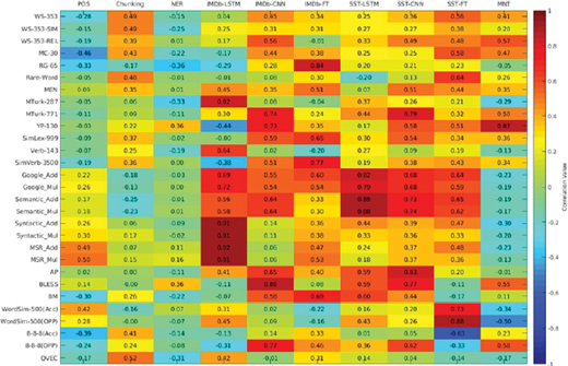
Pearson’s correlation between intrinsic and extrinsic evaluator, where the x-axis shows extrinsic evaluators while the y-axis indicates intrinsic evaluators. The warm indicates the positive correlation while the cool color indicates the negative correlation.
Fig. 1Close modalPearson’s correlation between intrinsic and extrinsic evaluator, where the x-axis shows extrinsic evaluators while the y-axis indicates intrinsic evaluators. The warm indicates the positive correlation while the cool color indicates the negative correlation.
We see from the correlation result that larger datasets tend to give more reliable and consistent evaluation result. Among all datasets, WS-353, WS-353-SIM, WS-353-REL, MTrurk-771, SimLex-999, and SimVerb-3500 are recommended to serve as generic evaluation datasets. Although datasets like MC-30 and RG-65also provide us with reasonable results, their correlation results are not as consistent as others. This may be attributed to the limited amount of testing samples with only dozens of testing word pairs. The RW dataset is a special one that focuses on low-frequency words and gains popularity recently. Yet, based on the correlation study, the RW dataset is not as effective as expected. Infrequent words may not play an important role in all extrinsic evaluation tasks. This is why infrequent words are often set to the same vector. The RW dataset can be excluded for general purpose evaluation unless there is a specific application demanding rare words modeling.
- •
Word analogy
The word analogy results are shown from the 14th row to the 21st row in the figure. Among four-word analogy datasets (i.e. Google, Google Semantic, Google Syntactic, and MSR), Google and Google Semantic are more effective. It does not make much difference in the final correlation study using either the 3CosAdd or the 3CosMul computation. Google Syntactic is not effective since the morphology of words does not contain as much information as semantic meanings. Thus, although the FastText model performs well in morphology testing based on the average of sub-words, its correlation analysis is worse than other models. In general, word analogy provides most reliable correlation results and has the highest correlation with the sentiment analysis task.
- •
Concept categorization
All three datasets (i.e. AP, BLESS, and BM) for concept categorization perform well. By categorizing words into different groups, concept categorization focuses on semantic clusters. It appears that models that are good at dividing words into semantic collections are more effective in downstream NLP tasks.
- •
Outlier detection
Two datasets (i.e. WordSim-500 and 8-8-8) are used for outlier detection. In general, outlier detection is not a good evaluation method. Although it tests semantic clusters to some extent, outlier detection is less direct as compared to concept categorization. Also, from the dataset point of view, the size of the 8-8-8 dataset is too small while the WordSim-500 dataset contains too many infrequent words in the clusters. This explains why the accuracy for WordSim-500 is low (around 10-20%). When there are larger and more reliable datasets available, we expect the outlier detection task to have better performance in word embedding evaluation.
- •
QVEC
QVEC is not ago ode valuator due to its in her it proper- ties. It attempts to compute the correlation with lexicon- resource-based word vectors. Yet, the quality of lexicon- resource-based word vectors is too poor to provide a reliable rule. If we can find a more reliable rule, the QVEC evaluator will perform better.
Based on the above discussion, we conclude that word similarity, word analogy, and concept categorization are more effective intrinsic evaluators. Different datasets lead to different performance. In general, larger datasets tend to give better and more reliable results. Intrinsic evaluators may perform very differently for different downstream tasks. Thus, when we test a new word embedding model, all three intrinsic evaluators should be used and considered jointly.
B) Consistency of extrinsic evaluators
For POS tagging, chunking, and NER, none of the intrinsic evaluators provide high correlation. Their performance depend on their capability in sequential information extraction. Thus, word meaning plays a subsidiary role in all these tasks. Sentiment analysis is a dimensionality reduction procedure. It focuses more on the combination of word meaning. Thus, it has a stronger correlation with the properties that the word analogy evaluator is testing. Finally, NMT is sentence-to-sentence conversion, and the mapping between word pairs is more helpful in translation tasks. Thus, the word similarity evaluator has a stronger correlation with the NMT task. We should also point out that some unsupervised machine translation tasks focus on word pairs [75,76]. This shows the significance of word pair correspondence in NMT.
IX. Conclusion and Future Work
In this work, we provided in-depth discussion of intrinsic and extrinsic evaluations on many word embedding models, showed extensive experimental results, and explained the observed phenomema. Our study offers a valuable guidance in selecting suitable evaluation methods for different application tasks. There are many factors affecting word embedding quality. Furthermore, there are still no perfect evaluation methods testing the word subspace for linguistic relationships because it is difficult to understand exactly how the embedding spaces encode linguistic relations. For this reason, we expect more work to be done in developing better metrics for evaluation on the overall quality of a word model. Such metrics must be computationally efficient while having a high correlation with extrinsic evaluation test scores. The crux of this problem lies in decoding how the word subspace encodes linguistic relations and the quality of these relations.
We would like to point out that linguistic relations and properties captured by word embedding models are different from how humans learn languages. For humans, a language encompasses many different avenues, e.g. a sense of reasoning, cultural differences, contextual implications, and many others. Thus, a language is filled with subjective complications that interfere with objective goals of models. In contrast, word embedding models perform well in specific applied tasks. They have triumphed over the work of linguists in creating taxonomic structures and other manually generated representations. Yet, different datasets and different models are used for different specific tasks.
We do not see a word embedding model that consistently performs well in all tasks. The design of a more universal word embedding model is challenging. To generate word models that are good at solving specific tasks, task-specific data can be fed into a model for training. Feeding a large amount of generic data can be inefficient and even hurt the performance of a word model since different task-specific data can lead to contending results. It is still not clear what is the proper balance between the two design methodologies.
Acknowledgements
Computation for the work was supported by the University of Southern California’s Center for High Performance Computing (hpc.usc.edu).
