


Research on graph representation learning has received great attention in recent years since most data in real-world applications come in the form of graphs. High-dimensional graph data are often in irregular forms. They are more difficult to analyze than image/video/audio data defined on regular lattices. Various graph embedding techniques have been developed to convert the raw graph data into a low-dimensional vector representation while preserving the intrinsic graph properties. In this review, we first explain the graph embedding task and its challenges. Next, we review a wide range of graph embedding techniques with insights. Then, we evaluate several stat-of-the-art methods against small and large data sets and compare their performance. Finally, potential applications and future directions are presented.
I. Introduction
Research on graph representation learning has gained more and more attention in recent years since most real-world data can be represented by graphs conveniently. Examples include social networks [1], linguistic (word co-occurrence) networks [2], biological networks [3], and many other multimedia domain-specific data. Graph representation allows the relational knowledge of interacting entities to be stored and accessed efficiently [4]. Analysis of graph data can provide significant insights into community detection [5], behavior analysis [6], and other useful applications such as node classification [7], link prediction [8], and clustering [9]. Various graph embedding techniques have been developed to convert the raw graph data into a high-dimensional vector while preserving intrinsic graph properties. This process is also known as graph representation learning. With a learned graph representation, one can adopt machine learning tools to perform downstream tasks conveniently.
Obtaining an accurate representation of a graph is challenging in three aspects. First, finding the optimal embedding dimension of representation [10] is not an easy task [11]. A representation of a higher dimension tends to preserve more information of the original graph at the cost of more storage requirement and computation time. A representation of a lower dimension is more resource efficient. It may reduce noise in the original graph as well. However, there is a risk of losing some critical information from the original graph. The dimension choice depends on the input graph type as well as the application domain [12]. Second, choosing the proper graph property to embed is an issue of concern if a graph has a plethora of properties. Graph characteristics can be reflected by node features, link structures, meta-data information, etc. Determining what kind of information is more useful is application dependent. For example, we focus more on the link structure in the friend recommendation application but more on the node feature in advertisement recommendation applications. For the former, the task is mainly grouping users into different categories to provide the most suitable service/goods. Third, many graph embedding methods have been developed in the past. It is desired to have some guidelines in selecting a suitable embedding method for a target application. In this paper, we will mainly focus on node prediction and vertex classification, which are widely used in real-world applications. We intend to provide an extensive survey on graph embedding methods with the following three contributions in mind:
We would like to offer new comers in this field a global perspective with insightful discussion and an extensive reference list. Thus, a wide range of graph embedding techniques, including the most recent graph representation models, are reviewed.
To shed light on the performance of different embedding methods, we conduct extensive performance evaluation on both small and large data sets in various application domains. To the best of our knowledge, this is the first survey paper that provides a systematic evaluation of a rich set of graph embedding methods in domain-specific applications.
We provide an open-source Python library, called the Graph Representation Learning Library (GRLL), to readers. It offers a unified interface for all graph embedding methods discussed in this paper. This library covers the largest number of graph embedding techniques until now.
The rest of this paper is organized as follows. We first state the problem as well as several definitions in Section II. Then, traditional and emerging graph embedding methods are reviewed in Section III. Next, we conduct extensive performance evaluation on a large number of embedding methods against different data sets in different application domains in Section V. The application of the learned graph representation and the future research directions are discussed in Sections VI and VII, respectively. Finally, concluding remarks are given in Section VIII.
II. Definition and Preliminaries
A) Notations
A graph, denoted by G = (V, E), consists of vertices, V = {v1, v2,…,v|v|}, and edges, E = {ei,j}, where an edge ei,j connects vertex vi to vertex vj. Graphs are usually represented by an adjacency matrix or a derived vector space representation [13]. The adjacency matrix, A, of graph G contains non-negative weights associated with each edge, aij ≥ 0. If vi and vj are not directly connected to one another, aij = 0. For undirected graphs, aij = aji for all 1 ≤ i ≤ j ≤ |V|.
Graph representation learning (or graph embedding) aims to map each node to a vector where the distance characteristics among nodes is preserved. Mathematically, for graph G = (V, E), we would like to find a mapping:
where d << |V|, and Xi = {x1, x2, …, xd} is the embedded (or learned) vector that captures the structural properties of vertex vi.
The first-order proximity [14] in a network is the pairwise proximity between vertices. For example, in weighted networks, the weights of the edges are the first-order proximity between vertices. If there is no edge observed between two vertices, the first-order proximity between them is 0. If two vertices are linked by an edge with a high weight, they should be close to each other in the embedding space. This objective can be obtained by minimizing the distance between the joint probability distribution in the vector space and the empirical probability distribution of the graph. If we use the KL-divergence [15] to calculate the distance, the objective function is given by:
where
and vi ∈ ℝd is the low-dimensional vector representation of vertex vi and wij is the edge weight between node i and j. vi, vj are the embeddings for node vi and vj.
The second-order proximity [16] is used to capture the two-step relationship between two vertices. Although there is no direct edge between two vertices of the second-order proximity, their representation vectors should be close in the embedded space if they share similar neighborhood structures.
The objective function of the second-order proximity can be defined as:
where
and is the vector representation of vertex vj when it is treated as a specific context for vertex vi.
Graph sampling is used to simplify graphs [17]. Sometimes, even if whole graph is known, we need to use sampling to obtain a smaller graph. If the graph is unknown, then sampling is regarded as a way to explore the graph. Commonly used techniques can be categorized into two types:
Negative sampling is proposed as an alternative to the hierarchical computation of the soft max. Computing soft max is expensive since the optimization requires the summation over the entire set of vertices. It is computationally expensive for large-scale networks. Negative sampling is developed to address this problem. It helps distinguish the neighbors from other nodes by sampling multiple negative samples according to the noise distribution. In the training process, correct surrounding neighbors are positive examples in contrast to a set of sampled negative examples (usually noise).
In the training stage, it is difficult to choose an appropriate learning rate in graph optimization when the difference between edge weights is large. To address this problem, one solution is to use edge sampling that unfolds weighted edges into several binary edges at the cost of increased memory. An alternative is treating weighted edges as binary ones with their sampling probabilities proportional to the weights. This treatment would not modify the objective function.
B) Graph embedding input
Graph embedding methods take a graph as the input, where the graph can be a homogeneous graph, a heterogeneous graph, a graph with/without auxiliary information, or a constructed graph [22]. They are detailed below:
Homogeneous graphs refer to graphs whose nodes and edges belong to the same type. All nodes and edges of homogeneous graphs are treated equally.
- Heterogeneous graphs contain different edge types to represent different relationships among different entities or categories. For example, their edges can be directed or undirected. Heterogeneous graphs typically exist in community-based question answering (cQA) sites, multimedia networks and knowledge graphs. Most social network graphs are directed graphs [23]. Only the basic structural information of input graphs is provided in real-world applications.Fig. 1
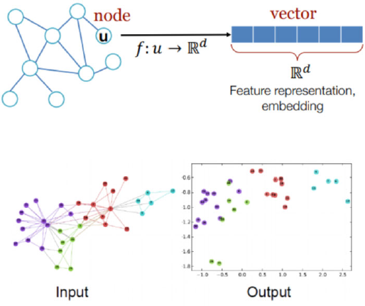
Illustration of graph representation learning input and output.
Graphs with auxiliary information [24, 25] are those that have labels, attributes, node features, information propagation, etc. A label indicates node’s category. Nodes with different labels should be embedded further away than those with the same label. An attribute is a discrete or continuous value that contains additional information about the graph rather than just the structural information. Information propagation indicates dynamic interaction among nodes, such as post sharing or “retweet” while Wikipedia [26], DBpedia [27], Freebase [28], etc.
Graphs constructed from non-relational data are assumed to lie in a low dimensional manifold. For this kind of graph, inputs are usually represented by feature matrix, X ∈ ℝ|V|×N, where each row Xi is a N-dimensional feature vector for the ith training instance. A similarity matrix, denoted by S, can be constructed by computing the similarity between Xi and Xj for graph classifications. An illustration of graph input and output is shown in Fig. 1.
C) Graph embedding output
The output of a graph embedding method is a set of vectors representing the input graph. Based on the need for specific application, different information or aspect of the graphs can be embedded. Graph embedding output could be node embedding, edge embedding, hybrid embedding, or whole-graph embedding. The preferred output form is application-oriented and task-driven, as elaborated below:
Node embedding represents each node as a vector, which would be useful for node clustering and classification. For node embedding, nodes that are close in the graph are embedded closer together in the vector representations. Closeness can be first-order proximity, second-order proximity or other similarity calculation.
Edge embedding aims to map each edge into a vector. It is useful for predicting whether a link exists between two nodes in a graph. For example, knowledge graph embedding can be used for knowledge graph entity/relation prediction.
Hybrid embedding is the combination of different types of graph components such as node and edge embedding. Hybrid embedding is useful for semantic proximity search and sub-graphs learning. It can also be used for graph classification based on graph kernels. Substructure or community embedding can also be done by aggregating individual node and edge embedding inside it. Sometimes, better node embedding is learned by incorporating hybrid embedding methods.
Whole graph embedding is usually done for small graphs such as proteins and molecules. These smaller graphs are represented as one vector, and two similar graphs are embedded to be closer. Whole-graph embedding facilitates graph classification tasks by providing a straightforward and efficient solution in computing graph similarities.
D) Overview of graph embedding ideas
The study of graph embedding can be traced back to 1900s when people questioned whether all planar graphs with n vertices have a straight line embedding in an nk × nk grid. This problem was solved in [30] and [31]. The same result for convex maps was proved in [32]. More analytic work on the embedding method and time/space complexity of such a method were studied in [33] and [34]. However, a more general approach is needed since most real-world graphs are not planer. A large number of methods have been proposed since then.
We provide an overview of various graph embedding ideas below:
Dimensionality reduction:
In early 2000s, graph embedding is achieved by dimensionality reduction. For a graph with n nodes, each of which is of dimension D. These embedding methods aim to embed nodes into a d-dimensional vector space, where d << D. They are called classical methods and reviewed in Section A. Dimensionality reduction is not very scalable, more advanced methods are needed for graph representation learning.
Random walk:
One can trace a graph by starting random walks from random initial nodes so as to create multiple paths. These paths reveal the context of connected vertices. The randomness of these walks gives the ability to explore the graph, capture the global and local structural information by walking through neighboring vertices. Later on, probability models like skip-gram and bag-of-word are performed on the randomly sampled paths to learn node representations. The random walk based methods will be discussed in Section III, B.
Matrix factorization:
By leverage the sparsity of real-world networks, one can apply the matrix factorization technique that finds an approximation matrix for the original graph. This idea is elaborated in Section III, C.
Neural networks:
Neural network models such as convolution neural network (CNN) [35], recursive neural networks (RNN) [36] and their variants have been widely adopted in graph embedding. This topic will be described in Section III, D.
Large graphs:
Some large graphs are difficult to embed since CNN and RNN models do not scale well with the numbers of edges and nodes. New embedding methods are designed targeting at large graphs. They become popular due to their efficiency. This topic is reviewed in Section III, E.
Hypergraphs:
Most social networks are hypergraphs. As social networks get more attention in recent years, hypergraph embedding becomes a hot topic, which will be presented in Section III, F.
Attention mechanism:
The attention mechanism can be added to existing embedding models to increase embedding accuracy, which will be examined in Section III, E.
An extensive survey on graph embedding methods will be conducted in the next section.
III. Graph Embedding Methods
A) Dimension-reduction-based methods
Classical graph embedding methods aim to reduce the dimension of high-dimensional graph data into a lower dimensional representation while preserving the desired properties of the original data. They can be categorized into linear and nonlinear two types. The linear methods include the following:
- 1
Principal component analysis (PCA) [37]:
The basic assumption for PCA is that that principal components that are associated with larger variances represent the important structure information while those smaller variances represent noise. Thus, PCA computes the low- dimensional representation that maximizes the data variance. Mathematically, it first finds a linear transformation matrix by solving4This equation aims to find the weight vector which extracts the maximum variance from this new data matrix, where Tr denotes the trace of a matrix, Cov(X) denotes the co-variance of data matrix X. D is the original dimension of the data, and d is the dimension the data are reduced to. It is well known that the principal components are orthogonal and they can be solved by eigen decomposition of the co-variance of data matrix [38].
- 2
Linear discriminant analysis (LDA) [39]:
The basic assumption for LDA is that each class is Gaussian distributed. Then, the linear projection matrix, W ∈ ℝD×d, can be obtained by maximizing the ratio between the inter-class scatter and intra-class scatters. The maximization problem can be solved by eigen decomposition and the number of low dimension d can be obtained by detecting a prominent gap in the eigen-value spectrum.
- 3
Multidimensional scaling (MDS) [40]:
MDS is a distance-preserving manifold learning method. It preserves spatial distances. MDS derives a dissimilarity matrix D, where Di,j represents the dissimilarity between points i and j, and produces a mapping in a lower dimension to preserve dissimilarities as much as possible.
The above-mentionedthree methods are referred to as “subspace learning” [11] under linear assumption. However, linear methods might fail if the underlying data are highly non-linear [41]. Then, non-linear dimensionality reduction (NLDR) [42] can be used for manifold learning. The objective is to learn the nonlinear topology automatically. The NLDR methods include the following:
Isometric feature mapping (Isomap) [43]:
The Isomap finds low-dimensional representation that most accurately preserves the pairwise geodesic distances between feature vectors in all scales as measured along the sub-manifold from which they were sampled. Isomap first constructs neighborhood graph on the manifold, then it computes the shortest path between pairwise points. Finally, it constructs low-dimensional embedding by applying MDS.
Locally linear embedding (LLE) [44]:
LLE preserves the local linear structure of nearby feature vectors. LLE first assigns neighbors to each data point. Then it computes the weights Wi,j that best linearly reconstruct the features, Xi, from its neighbors. Finally, it compute the low-dimensional embedding that best reconstructed by Wi,j. Besides NLDR, kernel PCA is another dimensionality reduction technique that is comparable to Isomap, LLE.
Kernel methods [45]:
Kernel extension can be applied to algorithms that only need to compute the inner product of data pairs. After replacing the inner product with kernel function, data are mapped implicitly from the original input space to a higher dimensional space. Then linear algorithms are applied in the new feature space. The benefit of kernel trick is that data which are not linearly separable in the original space could be separable in new high dimensional space. Kernel PCA is often used for NLDR with polynomial or Gaussian kernels.
B) Random-walk-based methods
Random-walk-based methods sample a graph with a large number of paths by starting walks from random initial nodes. These paths indicate the context of connected vertices. The randomness of walks gives the ability to explore the graph and capture both the global and the local structural information by walking through neighboring vertices. After the paths are built, probability models such as skipgram [46] and bag-of-words [47] can be performed on these randomly sampled paths to learn the node representation:
- 1
DeepWalk [48]:
DeepWalk is the most popular random-walk-based graph embedding method. In DeepWalk, a target vertex, v,, is said to belong to a sequence S = {v1,…, v|s|} sampled by random walks if v, can reach any vertex in S within a certain number of steps. The set of vertices, Vs = {Vi–t,…, Vi–1, Vi+1,…, Vi+t}, is the context of center vertex v’ with a window size of t (t is the sampling window size, which is a hyper parameter that can be tuned). DeepWalk aims to maximize the average logarithmic probability of all vertex context pairs in random walk sequence S. It can be written as:5where p(vj| vi) is calculated using the softmax function. It is proven in [49] that DeepWalk is equivalent to factorizing a matrix6each entry in M ∈ ℝ|V| × |V|, Mij, is the logarithm of the average probability that vertex Vi can reach vertex Vj in a fixed number of steps. W ∈ ℝk× |V| is the vertex representation. The information in H ∈ ℝk× |V| is rarely utilized in the classical DeepWalk model.
- 2
node2vec [50]:
node2vec is a modified version of DeepWalk. In DeepWalk, sampled sequences are based onthe depth-first sampling (DFS) strategy. They consist of neighboring nodes sampled at increasing distances from the source node sequentially. However, if the contextual sequences are sampled by the DFS strategy alone, only a few vertices close to the source node will be sampled. Consequently, the local structure will be easily overlooked. In contrast with the DFS strategy, the breadth-first sampling (BFS) strategy will explore neighboring nodes with a restricted maximum distance to the source node while the global structure may be neglected. As a result, node2vec proposes a probability model in which the random walk has a certain probability, 1 /p, to revisit nodes being traveled before. Furthermore, it uses an in-out parameter q to control the ability to explore the global structure. When the return parameter p is small, the random walk may get stuck in a loop and capture the local structure only. When in-out parameter q is small, the random walk is more similar to a DFS strategy and capable of preserving the global structure in the embedding space.
C) Matrix-factorization-based methods
Matrix-factorization-based embedding methods, also called graph factorization (GF) [51], was the first one to achieve graph embedding in O( |E|) time for node embedding tasks. To obtain the embedding, GF factorizes the adjacency matrix of a graph. It corresponds to a structure-preserving dimensionality reduction process. There are several variations as summarized below:
- 1
Graph Laplacian eigenmaps [52]:
This technique minimizes a cost function to ensure that points close to each other on the manifold are mapped close to each other in the low-dimensional space to preserve local distances.
- 2
Node proximity matrix factorization [53]:
This method approximates node proximity in a lowdimensional space via matrix factorization by minimizing the following objective function:7where Y is the node embedding and Yc is the embedding for the context nodes. W is the node proximity matrix, which can be derived by several methods. One way to obtain W is to use equation (6).
- 3
Text-associated DeepWalk (TADW) [49]:
TADW is an improved DeepWalk method for text data. It incorporates the text features of vertices in network representation learning via matrix factorization. Recall that the entry, mij, of matrix M ∈ ℝ|V|× |V| denotes the logarithm of the average probability that vertex vi randomly walks to vertex vij. Then, TADW factorizes Y into three matrices:8where and is the text feature matrix. In TADW, W and HT are concatenated as the representation for vertices.
- 4
Homophily, structure, and content augmented (HSCA) network [54]:
The HSCA model is an improvement upon the TADW model. It uses skip-gram and hierarchical Softmax to learn a distributed word representation. The objective function for HSCA can be written as9where ||.||2 is the matrix l2 norm and ||.||F is the matrix Frobenius form. In equation (9), the first term aims to minimize the matrix factorization error of TADW. The second term imposes the low-rank constraint on W and H and uses λ to control the trade-off. The last regularization term enforces the structural homophily between connected nodes in the network. The conjugate gradient (CG) [55] optimization technique can be used to update W and H. We may consider another regularization term to replace the third term; namely,10This term will make connected nodes close to each other in the learned network representation [56].
- 5
GraRep [57]:
GraRep aims to preserve the high order proximity of graphs in the embedding space. While the random-walk based methods have a similar objective, their probability model and objective functions used are difficult to explain how the high order proximity is preserved. GraRep derives a k-th order transition matrix, Ak, by multiplying the adjacency matrix to itself k times. The transition probability from vertex w to vertex c is the entry in the w-th row and c-th column of the k-th order transition matrix. Mathematically, it can be written as11With the transition probability defined in equation (11), the loss function is defined by the skip-gram model and negative sampling. To minimize the loss function, the embedding matrix can be expressed as12where β is a constant λ/N, λ is the negative sampling parameter, and N is the number of vertices. The embedding matrix, W, can be obtained by factorizing matrix Y in (12).
- 6
HOPE [58]:
HOPE preserves asymmetric transitivity in approximating the high order proximity, where asymmetric transitivity indicates a specific correlation among directed graphs. Generally speaking, if there is a directed edge from u to v, it is likely that there is a directed edge from v to u as well. Several high order proximities such as the Katz index [59], the Rooted Page-Rank, the Common Neighbors, and the Adamic-Adar were experimented in [58]. The embedding, vi, for node i can be obtained by factorizing the proximity matrix, S, derived from these proximities. To factorize S, SVD is adopted, and only the top-k eigenvalues are chosen.
D) Neural-network-based methods
Neural network models became popular again since 2010. Being inspired by the success of RNNs and CNNs, researchers attempt to generalize and apply them to graphs. Natural language processingmodels often use the RNNs to find a vector representation for words. The Word2Vec [60] and the skip-gram models [18] aim to learn the continuous feature representation of words by optimizing a neighborhood preserving likelihood function. Following this idea, one can adopt a similar approach for graph embedding, leading to the Node2Vec method [50]. Node2Vec utilizes random walks [61] with a bias to sample the neighborhood of a target node and optimizes its representation using stochastic gradient descent. Another family of neural- network-based embedding methods adopt CNN models. The input can be paths sampled from a graph or the whole graph itself. Some use the original CNN model designed for the Euclidean domain and reformat the input graph to fit it. Others generalize the deep neural model to non-Euclidean graphs.
Several neural-network-based methods based graph embedding methods are presented below:
- 1
Graph convolutional network (GCN) [62]:
GCN allows end-to-end learning of the graph with arbitrary size and shape. This model uses convolution operator on the graph and iteratively aggregates the embedding of neighbors for nodes. This approach is widely used for semi-supervised learning on graph- structured data. It is based on an efficient variant of convolutional neural networks that operate directly on graphs. GCN learns hidden layer representations that encode both local graph structure and features of nodes. In the first step of the GCN, a node sequence will be selected. The neighborhood nodes will be assembled, then the neighborhood might be normalized to impose the order of the graph, then convolutional layers will be used to learn the representation of nodes and edges. The propagation rule used is:13where A is the adjacency matrix, with enforced self loops to include the node features of itself, is the identity matrix. is the diagonal node degree matrix of . Under spectral graph theory of CNNs on graphs, GCN is equivalent to Graph Laplacian in the non-Euclidean domain [63]. The decomposition of eigenvalues for the normalized graph Laplacian data can also be used for tasks such as classification and clustering. GCN usually only uses two convolutional layers and why it works is not well explained. One recent work showed that GCN model is a special form of Laplacian smoothing [64, 65]. This is the reason that GCN works. Using more than two convolutional layers will lead to over-smoothing, therefore making the features of nodes similar to each other and more difficult to separate from each other.
- 2Signed graph convolutional network (SGCN) [66]: Most GCNs operate on unsigned graphs, however, many links in real-world have negative links. To solve this problem, signed GCNs aims to learn graph representation with the additional signed link information. Negative links usually contain semantic information that is different from positive links, also the principles are inherently different from positive links. The signed network will have a different representation as G = (V, ℰ+, ℰ–), where the signs of the edges are differentiated. The aggregation for positive and negative links are different. Each layer will have two representations, one for the balanced user where the number of negative links is even. One for the unbalanced user where the number of negative links is odd. The hidden states are:1415
where σ is the non-linear activation function, WB(l) and WU(l) are the linear transformation matrices for balanced and unbalanced sets.
- 3
Variational graph auto-encoders (VGAE) [67]:
VGAE uses an autoencoder minimizes the reconstruction error of the input and the output using an encoder and a decoder. The encoder maps input data to a representation space. Then, it is further mapped to a reconstruction space that preserves the neighborhood information. VGAE uses GCN as the encoder and an inner product decoder to embed graphs.
- 4
GraphSAGE [68]:
GraphSAGE uses a sample and aggregate method to conduct inductive node embedding. It uses node features such as text attributes, node profiles, etc. GraphSAGE trains a set of aggregation functions that integrate features of local neighborhood and pass it to the target node vi. Then, the hidden state of node vi is updated by:16where is the initial node attributes and ∑(·) denotes a certain aggregator function, e.g. average, LSTM, max-pooling, etc.
- 5Structural deep network embedding (SDNE) [69]: SDNE learns a low-dimensional network-structure preserving representation by considering both the first-order and the second-order proximities between vertexes using CNNs. To achieve this objective, it adopts a semi-supervised model to minimize the following objective function:17
where Lreg is an L2-norm regularizing term to avoid overfitting, S is the adjacency matrix, and B is the bias matrix.
E) Large graph embedding methods
Some large graphs are difficult to embed using the methods mentioned previously. Classical dimension reduction-based methods cannot capture the higher order proximity of large graphs, therefore cannot generate accurate representation. Most matrix factorization-based methods cannot take in large graph all at once, or has a high run time complexity. For example, graph Laplacian eigenmaps has the time complexity of O(|E|d2), making these methods not suitable for embedding large graphs. Random-walk based methods, such as Deep Walk, need to update parameters using back propagation (BP) [70], which is hardware demanding and time consuming. To address the scalability issue, several embedding methods targeting at large graphs have been proposed recently. They are examined in this subsection.
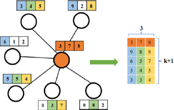
LGCL [29]:
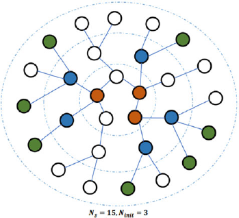
For each feature dimension, every node in the LGCL method selects a fixed number of features from its neighboring nodes with value ranking. Figure 2 serves as an example. Each node in this figure has a feature vector of dimension n=3. For the target node (in orange), the first feature component of its six neighbors takes the values of 9, 6, 5, 3, 0, and 0. If we set the window size to k=4, then the four largest values (i.e. 9,6,5, and 3) are selected. The same process is repeated for the two remaining features. By including the feature vector of the target node itself, we obtain a data matrix of dimension (k + 1) × n. This results in a grid-like structure. Then, the traditional CNN can be conveniently applied so as to generate the final feature vector. To embed large-scale graphs, a subgraph selection method is used to reduce the memory and resource requirements. As shown in Fig. 3, it begins with Ninit = 3 randomly sampled nodes (in red) that are located in the center of the figure. At the first iteration, the BFS is used to find all first-order neighboring nodes of initial nodes. Among them, Nm = 5 nodes (in blue) are randomly selected. At the next iteration, Nm = 7 nodes (in green) are randomly selected. After two iterations, 15 nodes are selected as a sub-graph that serves as the input to LGCL.
Graph partition neural networks (GPNN) [71]:
GPNN extends graph neural networks (GNNs) to embed extremely large graphs. It alternates between local (propagate information among nodes) and global information propagation (messages among sub-graphs). This scheduling method can avoid deep computational graphs required by sequential schedules. The graph partition is done using a multi-seed flood fill algorithm, where nodes with large out-degrees are sampled randomly as seeds. The sub-graphs grow from seeds using flood fill, which reaches out unassigned nodes that are direct neighbors of the current sub-graph.
LINE [23]:
LINE is used to embed graphs of an arbitrary type such as undirected, directed, and weighted graphs. It utilizes negative sampling to reduce optimization complexity.This is especially useful in embedding networks containing millions of nodes and billions of edges. It is trained to preserve the first- and second-order proximities, separately. Then, the two embeddings are merged to generate a vector space to better represent the input graph. One way to merge two embeddings is to concatenate embedding vectors trained by two different objective functions at each vertex.
F) Hyper-graph embedding
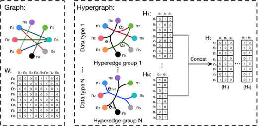
As research on social network embedding proliferates, a simple graph is not powerful enough to represent the information in social networks. The relationship of vertices in social networks is far more complicated than the vertex-to- vertex edge relationship. Different from traditional graphs, edges in hyper-graphs may have a degree larger than two. All related nodes are connected by a hyper-edge to form a super-node. Mathematically, an unweighted hyper-graph is defined as follows. A hyper-graph, denoted by G = (V, ℰ), consists of a vertex set V = {v1, v2,…, vn}, and a hyperedge set, E = {e1, e2,…, em}. A hyper-edge, e, is said to be incident with a vertex v if v ∈ e. When v ∈ e, the incidence function h(v, e) = 1. Otherwise, h(v, e) = 0. The degree of a vertex v is defined as . Similarly, the degree of a hyper-edge e is defined as . A hyper-graph can be represented by an incidence matrix H of dimension | V | × |ℰ | with entries h(v, e).
Hyper-edges possess the properties of edges and nodes at the same time. As an edge, hyper-edges connect multiple nodes that are closely related. A hyper-edge can also be seen as a super-node. For each pair of two super-nodes, their connection is established by shared incident vertices. As a result, hyper-graphs can better indicate the community structure in the network data. These unique characteristics of hyper-edges make hyper-graphs more challenging.
Comparison of properties of graphs and hyper-graphs
| Graph | Hyper-graph | |
|---|---|---|
| Representation | A(|V | × |V |) | H(|V | × |E |) |
| Minimum cut | NP-Hard | NP-Complete |
| Spectral clustering | Real-valued | Real-valued |
| optimization | optimization | |
| Spectral embedding | Matrix | Project to |
| factorization | eigenspace |
An illustration of graph and hyper-graph structures is given in Fig. 4. It shows how to express a hyper-graph in table form. The hyper-edges, which are indecomposable [72], can express the community structure of networks. Furthermore, properties of graphs and hyper-graphs are summarized and compared in Table 1. Graphs and hyper-graphs conversion techniques have been developed. Examples include clique expansion and star expansion. Due to the indecomposibility of hyper-edges, conversion from a hyper-graph to a graph will result in information loss.
Hyper-graph representation learning provides a good tool for social network modeling, and it has been a hot research topic nowadays. On the one hand, hyper-graph modeling can be used for many applications that are difficult to achieve using other methods. For example, multi-modal data can be better represented using hyper-graphs than traditional graph representation. On the other hand, hypergraphs can be viewed as a variant of simple graphs. Many graph embedding methods could be applied onto the hypergraphs with minor modifications. There are embedding methods proposed for simple graphs and they can be applied to hypergraphs as well as reviewed below:
- 1
Spectral hyper-graph embedding [74]:
Hyper-graph embedding can be treated as a k-way partitioning problem and solved by optimizing a combinatorial function. It can be further converted to a real-valued minimization problem by normalizing the hyper-graph Laplacian. Its solution is any lower dimension embedding space spanned by orthogonal eigen vectors of the hyper-graph Laplacian, ∆, with the k smallest eigenvalues.
- 2
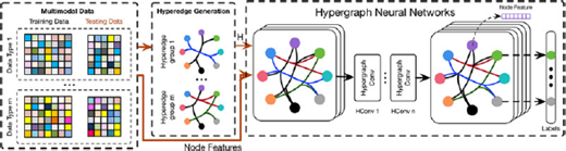
Hyper-graph neural network (HGNN) [73]:
Inspired by the spectral convolution on graphs in GCN [62], HGNN applies the spectral convolution to hyper-graphs. By training the network through a semisupervised node classification task, one can obtain the node representation at the end of convolutional layers. The architecture is depicted in Fig. 5. The hyper-graph convolution is derived from the hyper-graph Laplacian, ∆, which is a positive semi-definite matrix. Its eigen vectors provide certain basic functions while its associated eigenvalues are the corresponding frequencies. The spectral convolution in each layer is carried out via:18where X is the hidden embedding in each layer, Θ is the filter response, and Dv and De are diagonal matrices with entries being the degree of the vertices and the hyperedges, respectively.
- 3
Deep hyper-network embedding (DHNE) [72]:
DHNE aims to preserve the structural information of hyper-edges with a deep neural auto-encoder. The autoencoder first embed each vertex to a vector in a lower dimensional latent space and then reconstruct it to the original incidence vector. In the process of encoding and decoding, the second-order proximity is preserved to learn global structural information. The first order proximity is preserved in the embedding space by defining an N-tuple-wise similarity function. That is, if N nodes are in the same hyper-edge, the similarity of these nodes in the embedding space should be high. Based on similarity, one can predict whether N nodes are connected by a single hyper-edge. However, the N-tuple-wise similarity function should be non-linear; otherwise, it will lead to contradicted predictions. The local information of a hyper-graph can be preserved by shortening the distance of connected vertices in the embedding space.
G) Attention graph embedding
Attention mechanisms can be used to allow the learning process to focus on parts of a graph that are more relevant to a specific task. One advantage of applying attention to graphs is to avoid the noisy part of a graph so as to increase the signal-to-noiseratio [75] in information processing. Attention-based node embedding aims to assign an attention weight, αi ∈ [0, 1], to the neighborhood nodes of a target node t, where and N(t) denotes the set of neighboring nodes of t.
- 1
Graph attention networks (GAT) [76]:
GAT utilizes masked self-attentional layers to limit the shortcomings of prior graph convolutional based methods. They aim to compute the attention coefficients19where W is the weight matrix for the initial linear transformation, then the transformed information on each neighbor’s feature are concatenated to obtain the new hidden state, which will be passed through a LeakyReLu activation function, which is one of the most commonly used rectifiers. The above attention mechanism is a single-layer feed-forward neural network parameterized by the above weight vector.
- 2Generally speaking, one can use the random walk to find the context of the node. For a graph, G, with corresponding transition matrix T and window size c the parameterized conditional expectation after a k-step walk can be expressed as:20
where In is the size-n identity matrix, qk, 1 ≤ i ≤ c, are the trainable weights, D is the walk distribution matrix whose entry Duv encodes the number of times node u is expected to visit node v. The trainable weights are used to steer the walk toward a broader neighborhood or restrict it within a smaller neighborhood. Following this idea, Attention Walks adopts an attention mechanism to guide the learning procedure. This mechanism suggests which part of the data to focus on during the training process. The weight parameters are called the attention parameters in this case.
- 3
Attentive graph-based recursive neural network (AGRNN) [79]:
AGRNN applies attention to a graph-based recursive neural network (GRNN) [80] to make the model focus on vertices with more relevant semantic information. It builds sub-graphs to construct recursive neural networks by sampling a number of k-step neighboring vertices. AGRNN finds a soft attention, αr, to control how neighbor information should be passed to the target node. Mathematically, we have:21where xk is the input, W(a) is the weight to learn, and hr is the hidden state of the neighbors. The aggregated representation from all neighbors is used as the hidden state of the target vertex:22where N (vk) denotes the set of neighboring nodes of vertex vk. Although attention has been proven to be useful in improving some neural network models, it does not always increase the accuracy of graph embedding [81].
H) Others
- 1
GraphGAN [82]:
GraphGAN employs both generative and discriminative models for graph representation learning. It adopts adversarial training and formulates the embedding problem as a mini-max game, borrowing the idea from the generative adversarial network (GAN) [83]. To fit the true connectivity distribution ptrue(v|vc) of vertices connected to target vertex vc, GraphGAN models the connectivity probability among vertices in a graph with a generator, G(v|vc; θG), to generate vertices that are most likely connected to vc. A discriminator D(v, vc; θD) outputs the edge probability between v and vc to differentiate the vertex pair generated by the generator from the ground truth.
The final vertex representation is determined by alternately maximizing and minimizing the value function V(G, D) as:23 - 2
GenVector [26]:
GenVector leverages large-scale unlabeled data to learn large social knowledge graphs. This is a weakly supervised problem and can be solved by unsupervised techniques with a multi-modal Bayesian embedding model. GenVector can serve as a generative model in applications. For example, it uses latent discrete topic variables to generate continuous word embeddings, graph-based user embeddings, and integrates the advantages of topic models and word embeddings.
IV. Comparison of Different Methods and Applications
Classical dimensionality reduction methods have been widely used in graph embedding. They are mathematically transparent, yet most of them cannot represent the high order proximity in graphs. DeepWalk-based methods do not attempt to embed the whole graph but sample the neighborhood information of each node statistically. On the one hand, they can capture the long-distance relationship among nodes. On the other hand, the global information of a graph may not be fully preserved due to sampling. Matrix factorization methods find the graph representation based on the statistics of pairwise similarities. Such methods can outperform deep-learning method built upon random walk methods, where only a local context window is used. However, matrix factorization can be inefficient and unscalable for large graphs. This is because proximity matrix construction as well as eigen decomposition demand higher computational and storage complexities. Moreover, factorization methods such as LLE, Laplacian Eigenmaps and Graph Factorization only conserve the first order proximity. The LLE method has a time complexity of O(Ed2) while the GF has a time complexity of O(Ed), where d is the number of dimensions. In contrast, random walks usually have a time complexity O( | V | d). Moreover, factorization based method usually such as LLE, Laplacian Eigenmaps, and Graph Factorization only conserves first order proximity while DeepWalk-based methods can conserve second order proximity.
Deep learning architectures are mostly built upon neural networks. Such models rely heavily on modern GPU to optimize the parameters. They can preserve higher order proximities. Most state-of-the-art applications are based on such models. However, they are mathematically intractable and difficult to interpret. Besides, the training of model parameters with BP demands high time complexity. Large graph embedding methods such as LGCL and GPNN can handle larger graphs. They are suitable for the embedding of social networks, which contain thousands or millions of nodes. However, there are several limitations on these methods. First, these methods have a high time complexity. Second, graphs are dynamic in nature. Social network graphs and citation graphs in academic database are changing from time to time, and the graph structure keep growing over time. However, these methods usually work on static graphs. Third, they demand the pre-processing of the raw input data. It is desired to develop scalable embedding techniques.
Hyper graph embedding can be used to model more complex data and more dynamic networks, they are powerful in representing the information of social networks. However, they are more difficult to implement. Other methods provide alternatives for graph embedding but have not been used widely. Most of them are still in the “proof- of-concept” stage. Kernel methods convert a graph into a single vector. The resulting vector can facilitate graph level analytical tasks such as graph classification. They are more efficient than deep network models since they only need to enumerate the desired atomic substructures in a graph. However, they have a redundant substructure in the graph representation. Also, the embedding dimension can grow exponentially. Generative models leverage the information from different aspects of the graph such as graph structure, node attribute, etc. in a unified model. However, modeling observations based on the assumption of certain distributions is difficult to justify. Furthermore, generative models demand a large amount of training data to fit the data, which might not work well for small graphs.
All the methods mentioned above are summarized in Table 2.
V. Evaluation
We study the evaluation of various graph representation methods in this section. Evaluation tasks and data sets will be discussed in Sections A and B, respectively. Then, evaluation results will be presented and analyzed in Section C.
A) Evaluation tasks
The two most common evaluation tasks are vertex classification and link prediction. We use vertex classification to compare different graph embedding methods and draw insights from the obtained results.
Vertex classification:
Vertex classification aims to assign a class label to each node in a graph based on the information learned from other labeled nodes. Intuitively, similar nodes should have the same label. For example, closely-related publication may be labeled as the same topic in the citation graph while individuals of the same gender, similar age, and shared interests may have the same preference in social networks. Graph embedding methods embed each node into a low-dimensional vector. Given an embedded vector, a trained classifier can predict the label of a vertex of interest, where the classifier can be support vector machine (SVM) [84], logistic regression [85], kNN (k nearest neighbors) [86], etc. The vertex label can be obtained in an unsupervised or semi-supervised way. Node clustering is an unsupervised method that groups similar nodes together. It is useful when labels are unavailable. The semi-supervised method can be used when part of the data are labeled. The F1 score is used for evaluation in binary-class classification, while the micro-F1 score is used in multi-class classification. Since accurate vertex representations contribute to high classification accuracy, vertex classification can be used to measure the performance of different graph embedding methods.
Table 2Summary of different graph embedding methods
Category Example algorithm Advantage Disadvantage Dimension reduction based PCA, LDA, MDS, Isomap, LLE, Kernel methods Mathematicallytractable, well understood and easy to implement Cannot capture higher order proximity well Random walk based DeepWalk, node2vec Does not take the whole graph at once Sometimes cannot capture global information very well Matrix factorization based Graph Laplacian Eigenmaps, Node proximity Matrix Factorization, TADW, HSCA, GraRep, HOPE Can capture global structure High time complexity Neural network based GCN, SGCN, VGAE, GraphSAGE, SDNE, State-of-the-art performance Hardware demanding,training with BP is time consuming Large graph embedding Hyper Graph Embedding LGCL, GPNN, LINE Spectral Hyper-graphembedding, HGNN, DHNE Good scalability Can model more complex data High time complexity More difficult to implement Attention graph embedding Others GAT, Attention Walks, AGRNN GraphGAN, GenVector Better long distance node modeling Provide more alternatives High time complexity Proof-of-concept stage Link prediction [87]:
Link prediction aims to infer the existence of relationship or interaction among pairs of vertices in a graph. The learned representation should help infer the graph structure, especially when some links are missing. For example, links might be missing between two users and link prediction can be used to recommend friends in social networks. The learned representation should preserve the network proximity and the structural similarity among vertices. The information encoded in the vector representation for each vertex can be used to predict missing links in incomplete networks. The link prediction performance can be measured by the area under curveor the receiver operating characteristiccurve. A better representation should be able to capture the connections among vertices better.
We describe the benchmark graph data sets and conduct experiments in vertex classification on both small and large data sets in the following subsections.
B) Evaluation data sets
Citation data sets such as Citeseer [88], Cora [89], and PubMed [90] are examples of small data sets. They can be represented as directed graphs in which edges indicates author-to-author or paper-to-paper citation relationship and text attributes of paper content at nodes.
First, we describe several representative citation data sets below:
Citeseer [88]:
It is a citation index data set containing academic papers of six categories. It has 3312 documents and 4723 links. Each document is represented by a 0/1-valued word vector indicating the absence/presence of the corresponding word from a dictionary of 3703 words. Thus, the text attributes of a document is a binary-valued vector of 3703 dimensions.
Cora [89]:
It consists of 2708 scientific publications of seven classes. The graph has 5429 links that indicate citation relations between documents. Each document has text attributes that are expressed by a binary-valued vector of 1433 dimensions.
Wikipedia [91]:
The Wikipedia is an online encyclopedia created and edited by volunteers around the world. The data set is a word co-occurrence network constructed from the entire set of English Wikipedia pages. This data contains 2405 nodes, 17981 edges and 19 labels.
Next, we present several commonly used large graph data sets below:
BlogCatalog [92]:
It is a network of social relationships of bloggers listed in the BlogCatalog website. The labels indicate blogger’s interests inferred from the meta-data provided by bloggers. The network has 10 312 nodes, 333 983 edges and 39 labels.
YouTube [93]:
It is a social network of YouTube users. This graph contains 1 157 827 nodes, 4 945 382 edges and 47 labels. The labels represent groups of users who enjoy common video genres.
Flickr [94]:
It is an online photo management and sharing data set. It contains 80 513 nodes, 5 899 882 edges and 195 labels.
Summary of representative graph data sets
| No. of nodes | No. of edges | No. of classes | |
|---|---|---|---|
| Citeseer | 3312 | 4723 | 6 |
| Cora | 2708 | 5429 | 7 |
| Wiki | 2405 | 17 981 | 19 |
| BlogCatalog | 10 312 | 333 983 | 39 |
| YouTube | 1 157 827 | 4 945 382 | 47 |
| Flickr | 80 513 | 5 899 882 | 195 |
Finally, the parameters of the above-mentioned data sets are summarized in Table 3.
C) Evaluation results and analysis
Since evaluations were often performed independently on different data sets under different settings in the past, it is difficult to draw a concrete conclusion on the performance of various graph embedding methods. Here, we compare the performance of graph embedding methods using a couple of metrics under the common setting and analyze obtained results. In addition, we provide an open-source Python library, called the graph representation learning library (GRLL), to readers in the Github. It offers a unified interface for all graph embedding methods that were experimented in this work. To the best of our knowledge, this library covers the most significant number of graph embedding techniques until now.
1) Vertex classification
We compare vertex classification accuracy of seven graph embedding methods on Cora, Citeseer, and Wiki. We used the default hyper-parameter setting provided by each graph embedding method. For the classifier, we adopt linear regression forall methods(except forGCN sinceitisasemi- supervised algorithm). We randomly split samples equally into the training and the testing sets (i.e. 50 and 50%). The default embedding size is 128. The vertex classification results are shown in Table 4. DeepWalk and node2vec offer the highest accuracy for Cora and Wiki, respectively. The graph convolutional methods (i.e. GCN) yields the best accuracies in all three data sets because it uses multiple layers of graph convolution to propagate information between nodes. The connectivity information is therefore interchanged and is useful for vertex classification. The random-walk-based methods (e.g. DeepWalk, node2vec, and TADW) also get superior performance since they are able to capture the contextual information in graphs. In Wiki, data set, the node features are not given so it’s initialized as an identity matrix. Therefore, TADW couldn’t get comparable performance as other methods, demonstrating that good initial attributes for nodes is important for vertex classification. DeepWalk and node2vec are preferred among random-walk-based methods since TADW usually demands initial node features and much more memory. However, if the initial node attributes are presented, TADW could get better results than simple random-walk based methods.
Performance comparison of nine common graph embedding methods in vertex classification on Cora, Citeseer, and Wiki
| Cora | Citeseer | Wiki | |
|---|---|---|---|
| DeepWalk [48] | 0.829 | 0.592 | 0.670 |
| node2vec [50] | 0.803 | 0.597 | 0.680 |
| GraRep [57] | 0.787 | 0.535 | 0.650 |
| HOPE [58] | 0.646 | 0.422 | 0.608 |
| SDNE [69] | 0.573 | 0.427 | 0.510 |
| LINE [23] | 0.762 | 0.493 | 0.646 |
| GF [53] | 0.573 | 0.391 | 0.581 |
| TADW [49] | 0.852 | 0.734 | 0.411 |
| GCN [62] | 0.875 | 0.740 | 0.686 |
2) Visualization
Visualizing the embedding is useful to understand how well the embedding methods learn from the graph structure and node attributes. To be considered as good representation, vectors for nodes in the same class should have shorter distance and higher similarity to each other. Meanwhile, vectors for nodes from different classes should be as separable as possible so the downstream machine learning models will be able to obtain better performance. To visualize high-dimensional vectors, we adopt a widely-used dimension reduction algorithms, t-SNE [95], to transform the high-dimensional vectors to a two-dimensional space for visualization. We visualized three major branches of graph embedding learning methods, which are random-walkbased (DeepWalk), structural-preservation-based (LINE), and neural-network-based methods (SDNE). We choose Cora as the data set to be tested. The results are shown in Fig. 6. The random-walk-based method provides separable inter-class representation by capturing the contextual information in the graphs. Nodes that don’t appear in the same context tend to be separated. However, the intra-class vectors are not clustered well due to the randomly sampled paths. The structural-preservation-based method provides the most compact intra-class clusters due to preservation of the first and second order proximity. The graph structure can be reflected the most by this category of methods. The representation vectors from the neural-network-based method are mainly located on a high-dimensional manifold in the latent space. The arrangement of the embedding is often uneven and biased.The authors in [96] discussed this effect and proposed a post-processing scheme to solve the problem. Consequently, the representation vectors from the neural-network-based method are nearly not linearly- separable.
3) Clustering quality
We compare various graph embedding methods by examining their clustering quality in terms of the macro and micro-Fı scores. The K-means++ algorithm is adopted for the clustering task. Since the results of K-means++ clustering are dependent upon seed initialization, we perform 10 consecutive runs and report the best result. We tested them on three large graph data sets (i.e. YouTube, Flickr, and BlogCatalog). The experimental results are shown in Table 6. YouTube and Flickr contain more than millions of nodes and edges and we can only run DeepWalk, node2vec, and LINE on them with the 24G RAM limit as reported in the table. We see that DeepWalk and node2vec provide the best results. They are both random-walk based methods with different sampling schemes. Also, they demand less memory as compared with others. In general, random walk with the skip-gram model is a good baseline for unsupervised graph embedding. GraRep offers a comparable graph embedding quality for BlogCatalog. However, its memory requirement is significant so that it is not suitable for large graphs.
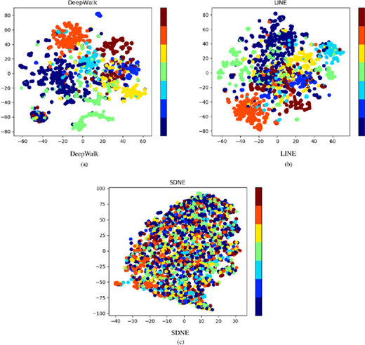
t-SNE visualization of different embedding methods on Cora. The seven different colors of points represent different classes of the nodes.
t-SNE visualization of different embedding methods on Cora. The seven different colors of points represent different classes of the nodes.
4) Time complexity
Time complexity is an essential factor to consider, which is especially true for large graphs. The time complexity of three embedding methods (DeepWalk, node2vec, and LINE) against three data sets (YouTube, Flickr, and Wiki) is compared in Table 5. Three embedding methods all apply negative sampling [18] to reduce the time complexity. We observe that the training time of DeepWalk is significantly lower than node2vec and LINE for larger graph data sets such as YouTube and Flickr. DeepWalk is an efficient graph embedding method with high accuracy by considering embedding quality as well as training complexity.
Comparison of time used in training (s)
| YouTube | Flickr | Wiki | |
|---|---|---|---|
| DeepWalk | 37 366.00 | 3636.14 | 37.23 |
| node2vec | 41626.94 | 40 779.22 | 27.53 |
| LINE | 185153.29 | 31 707.87 | 79.42 |
Comparison of clustering quality of six graph embedding methods in terms of macro- and micro-F1 scores against three large graph data sets
| DeepWalk | node2vec | LINE | GraRep | GF | HOPE | ||
|---|---|---|---|---|---|---|---|
| YouTube | Macro-F1 | 0.206 | 0.221 | 0.170 | N/A | N/A | N/A |
| Micro-F1 | 0.293 | 0.301 | 0.266 | N/A | N/A | N/A | |
| Flickr | Macro-F1 | 0.212 | 0.203 | 0.162 | N/A | N/A | N/A |
| Micro-F1 | 0.313 | 0.311 | 0.289 | N/A | N/A | N/A | |
| BlogCatalog | Macro-F1 | 0.247 | 0.250 | 0.194 | 0.230 | 0.072 | 0.143 |
| Micro-F1 | 0.393 | 0.400 | 0.356 | 0.393 | 0.236 | 0.308 |
5) Influence of embedding dimensions
As the embedding dimension decreases, less information about the input graph is preserved so that the performance drops. However, some methods will be affected by the decrease of embedding size than others. We show the node classification accuracy as a function of the embedding dimension for the Cora and Citeseer data set in Fig. 7. We compare eight graph embedding methods (DeepWalk, node2vec, GraRep, HOPE, SDNE, LINE, GF, and TADW) and their embedding dimensions vary from 4, 8, 16, 32, 64 to 128. The experimental results are shown in Fig. 7. We see that the performance of the random-walk based embedding methods (Deep-Walk and node2vec) degrades slowly. Only about 10% drop in performance when the embedding dimension size drops from 128 to 4. An exception is TADW, which requires initial node features to obtain the final embedding. The initial attributes are usually sparse and high dimensional, transforming them to a lower-dimensional embedding space will cause great information loss. In contrast, the performance of the structure preserving methods (LINE and GraRep) drops significantly (as much as 45%) when the embedding size goes from 128 to 4. One explanation is that the structural preserving methods are compressing the adjacency matrix into a lower dimensional space. When the compression ratio is higher, the distortion will be higher as well. Random-walk based methods obtain embedding vectors by selecting paths from the input graph randomly. Yet, the relationship between nodes is still preserved when the embedding dimension is small. SDNE adopts the auto-encoder architecture to preserve the information of the input graph so that its performance remains about the same regardless of the embedding dimension.
6) Influence of training sample ratio
By the training sample ratio, we mean the percentages of total node samples that are used for the training purpose. When the ratio is high, the classifier could be overfitted. On the other hand, if the ratio is too low, the offered information may not be sufficient for the training purpose. Such analysis is classifier dependent, and we adopt a simple linear regression classifier from the python sklearn toolkit in the experiment. The node classification accuracy as a function of the training sample ratio for the Cora and Citeseer data set is shown in Fig. 8. Most methods have consistent performance for the training data ratio between 0.2 and 0.8 except for the deep learning based methods (SDNE). Its accuracy drops when the training data ratio is low. It needs a higher ratio of training data. GCN uses multiple graph convolutional layers to propagate information between neighboring nodes so it could get good performance with smaller training set. However, when the training ratio becomes higher, the accuracy for GCN would not increase much or even drop due to over-fitting.
VI. Emerging Applications
Graphs offer a powerful modeling tool and find a wide range of applications. Since many real-world data have some certain relationships among entities, they can be conveniently modeled by graphs. Multi-modal data can also be embedded into the same space through graph representation learning and, as a result, the information from different domains can be represented and analyzed in one common setting.
In this section, we examine three emerging areas that benefit from graph embedding techniques.
Community detection:
Graph embedding can be used to predict the label of a node given a fraction of labeled node [13, 97-99]. Thus, it has been widely used for community detection [100, 101]. In social networks, node labels might be gender, demography, or religion. In language networks, documents might be labeled with categories or keywords. Missing labels can be inferred from labeled nodes and links in the network. Graph embedding can be used to extract node features automatically based on the network structure and predict the community that a node belongs to. Both vertex classification [102] and link prediction [103, 104] can facilitate community detection [105, 106].
Recommendation system:
Recommendation is an important function in social networks and advertising platforms [107-109]. Besides the structure, content and label data [110], some networks contain spatial and temporal information. For example, Yelp may recommend restaurants based on a user’s location and preference. Spatial-temporal embedding [111] is an emerging topic in mobile applications.
Graph compression and coarsening:
By graph compression (graph simplification), we refer to a process of converting one graph to another, where the latter has a smaller number of edges. Graph coarsening can be used for compression, which is a method used to partition a graph in multiple stages. Graph coarsening is usually used in the first stage for graph embedding. It works by collapsing pairs of nodes and edges using a determinate criteria. Graph coarsening is useful because the size of the graphs may be too big to be partitioned. Graph compression aims to store a graph more efficiently and run graph analysis algorithms faster. For example, a graph is partitioned into bipartite cliques and replaced by trees to reduce the edge number in [112]. Along this line, one can also aggregate nodes or edges for faster processing with graph coarsening [113], where a graph is converted into smaller ones repeatedly using a hybrid matching technique to maintain its backbone structure. The structural equivalence matching (SEM) method [114] and the normalized heavy edge matching method (NHEM) [115] are two examples.Fig. 7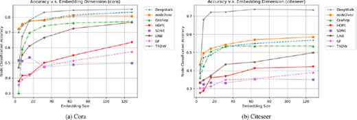
The node classification accuracy as a function of the embedding size.
Fig. 8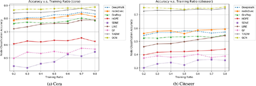
The node classification accuracy as a function of the embedding size.
Biomedical application:
Graph representation learning can be used to for biomedical data analysis. For example, brain network data can be modeled through the graph, with the brain activities as signals residing on the nodes [116]. The embedding methods can be used for studying the structures and functions of brains when under different stimuli. Some frameworks have been proposed for studying Alzheimer’s disease [117], and brain reaction to magnetoencephalographysignals [118].
Other application domain:
Graph learning can also be applied to meteorology for studying networks of weather stations. The authors in [119, 120] aim to capture the relationship among different weather stations in terms of their attitude. It is still in the stage of proof of concept and more research is needed. Graph embedding can also be used in traffic flow inference [121], Internet news propagation study [122], inter-region political relationship [120], human robotics interaction [123],ontologies of concepts [124], etc.
VII. Future Research Directions
Graph representation learning is a well-motivated topic. It is an effective way to convert graph data into a low dimensional space [125, 126] in which important feature information are well preserved. Graph analytic can provide researchers with a deeper understanding of the data with the help of efficient graph embedding techniques. Based on the discussion above, we would like to discuss several future research opportunities in graph embedding.
Deep graph embedding:
GCN [62] and some of its adaptation [123] has drawn great attention due to its superior performance. However, the number of graph convolutional layers is typically not higher than two. When there are more graph convolutional layers in cascade, the performance drops significantly. It was argued in [65] that each GCN layer corresponds to graph Laplacian smoothing since node features are propagated in the spectral domain. When a GCN is deeper, the graph Laplacian is over-smoothed and the corresponding node features become obscure. Each layer of GCN usually only learns one-hop information, and two GCN layers learn the first- and second- order proximity in the graph. It is difficult for a shallow structure to learn global information. One solution to fix this problem is to conduct the convolution in the spatial domain. For example, one can convert graph data into grid-structure data as proposed in [29]. Then, the graph representation can be learned using multiple CNN layers. Another way to address the problem is to down-sample graphs and merge similar nodes. Such a graph coarsening idea was adopted by [127-129] to build deep GCNs. Then, we can build a hierarchical network structure, which allows us to learn both local and global graph data in a hierarchical manner.
Dynamic graph embedding:
Social graphs, such as graphs in Twitter, are always changing. Another example is graphs of mobile users whose location information is changing along with time. To learn the representation of dynamic graphs is an important research topic and it finds applications in realtime and interactive processes such as the optimal travel path planning in a city at traffic hours. Hyper-graphs is a good option for modeling such dynamics in graphs. Embed the time sequence into each node can also be useful; for example, long-short-term-memory (LSTM) can be used on each vertex to incorporate sequential changes.
Scalability of graph embedding:
With the rapid growth of social networks, which contain millions and billions of nodes and edges, We expect to see graphs of a larger scale and higher diversity. How to embed enormous graph data efficiently and accurately is still an open problem. Deep neural network models have the state-of-the-art performance. However, these methods suffer the low efficiency problem. They rely on modern GPU to find the optimal parameters. Better paradigms are needed for processing large-scale graphs. One possibility is to use a feedforward machine-learning design to process the graph without BP. Another option is to use better graph coarsening or partitioning method to preprocess the data.
Interpretability of graph embedding:
Most state-of-the-art graph embedding methods are built upon CNNs, which are trained with BP to determine their model parameters. However, the training complexity is very high. Some research was performed to lower the training complexity such as quickprop [130]. However, training model parameters iteratively using BP is still time consuming and hardware demanding. In addition, CNNs are mathematically intractable. Very recently, some researchers have tried to explain the interpretability of neural network models [131, 132]. The authors in [133] attempt to explain CNNs using an interpretable and feedforward (FF) design without any BP. The work in [133] adopts a FFdata-centric approach to network parameters of the current layer based on data statistics from the output of the previous layer in a one-pass manner. It would be worthwile to apply FF machine-learning methods to graph embedding tasks. An interpretable design as an alternative to advanced neural network architectures can shed light on current graph embedding-related machine-learning research.
VIII. Conclusion
A comprehensive survey of the literature on graph representation learning techniques was conducted in this paper. We examined various graph embedding techniques that convert the input graph data into a low-dimensional vector representation while preserving intrinsic graph properties. Besides classical graph embedding methods, we covered several new topics such as neural-network-based embedding methods, hypergraph embedding and attention graph embedding methods. Furthermore, we conducted an extensive performance evaluation of several stat-of-the- art methods against small and large data sets. For experiments conducted in our evaluation, an open-source Python library, called the GRLL, was provided to readers. Finally, we presented some emerging applications and future research directions. We hope our work can inspire more follow-up work in graph embedding.
