


In a first of its kind, this paper tries to explore the long-run relationship between investors' sentiment and selected industries' returns over the period January 2010 to December 2021.
The paper uses 23 market and macroeconomic proxies to measure investor sentiment. Principal component analysis has been used to create sentiment sub-indices that represent investor sentiment. The autoregressive distributed lag (ARDL) model and other sophisticated econometric techniques such as the unit root test, the cumulative sum (CUSUM) stability test, regression, etc. have been used to achieve the objectives of the study.
The authors find that there is a significant relationship between sentiment sub-indices and industries' returns over the period of study. Market and economic variables, market ratios, advance-decline ratio, high-low index, price-to-book value ratio and liquidity in the economy are some of the significant sub-indices explaining industries' returns.
The study has relevant implications for retail investors, policy-makers and other decision-makers in the Indian stock market. Results are helpful for the investor in improving their decision-making and identifying those sentiment sub-indices and the variables therein that are relevant in explaining the return of a particular industry.
The study contributes to the existing literature by exploring the relationship between sentiment and industries' returns in the Indian stock market and by identifying relevant sentiment sub-indices. Also, the study supports the investors' irrationality, which arises due to a plethora of behavioral biases as enshrined in classical finance.
1. Introduction
Economic literature assumes that economic events can be described using efficient and controlled models. Human beings are part of this reality and being the most complex creature in this world, it is very difficult to explain and predict the events. Till now, efforts are being made to recognize and describe the functioning of human minds. On the basis of this, it can be said that assumptions about investors’ rationality, market efficiency and fast decision-making are totally false. Most of the economic and financial models ignore the behavioral aspect of decision-making, but authors strongly believe that considering behavioral aspects can help in a better understanding of decision-making, especially in the context of the stock market.
Classical finance supports the rationality of investors and behavioral finance is a response to this rationality and aims at predicting the market on the basis of understanding the sentiment of investors. Baker and Wurgler (2006) define sentiment as the erroneous or biased beliefs of the investors about future cash flows and risk which is unpredictable. Behavioral finance literature suggests that investors do not follow rationality completely. Normal and systematic cognitive biases present in the course of decision-making encourage investors to invest on the basis of their instincts and not the fundamentals.
Following the above arguments, behavioral approaches to asset pricing try to integrate investor sentiment as an additional source of risk. The major drive in this respect is to show the fact that the expected return of a security is a combination of fundamental components and sentiment premium (Shefrin, 2008).
Today, investor sentiment is playing an important role as a cornerstone of modern behavioral finance. Investor sentiment is not impossible to measure, but it is definitely difficult. The authors proposed that either a survey method can be used or proxies to the sentiment can be used to measure the sentiment.
When investors are optimistic then there is an increase in the returns and vice-versa. Though the existing literature supports the implication of sentiment on asset pricing, there is one issue that doubts the generalization of the sentiment. Most of the studies are devoted to the understanding relationship between sentiment and aggregate return of the market. Few studies have tried to understand the relationship between sentiment and return at the industry level, especially in the context of the Indian stock market (Dash & Mahakud, 2013b). Assuming when sentiment is high then investors buy more stocks, we propose that sentiment affects different industries differently. Further, the factors responsible for the high/low sentiment may also be different for different industries.
Keeping the above arguments in mind, our objectives are as follows:
To evaluate the sentiment of Indian investors using proxies to it.
To analyze the impact of sentiment on the return of select Indian industries.
We expect that sentiment affects the industries’ return. Above analysis will help to get insights into the sentiment sub-indices which can explain the return of industries under consideration.
2. Review of literature
The sentiment is a personal belief or judgment that is not based on evidence or certainty. Sentiment is an important term used frequently in the field of behavioral sciences and finance. According to Keynes (1936), sentiment is nothing but the animal spirits of human beings which they show while making financial decisions. Zweig (1973) defined sentiment as something which belongs to the perceptive comparisons of the investment made by the investors. Lee, Shleifer, and Thaler (1991) supported the above view and claimed that predicting the return using sentiment incorporation of economic fundamentals is not sufficient. One of the dimensions of the sentiment is the propensity of investors to gamble in the financial market (Baker & Wurgler, 2006). Smidt (1968) and Baker, Wurgler, and Spring (2007) supported the above dimension and claimed that investors speculate in the market due to the existence of sentiment. Sehgal, Sood, and Rajput (2009) defined the sentiment and identified the factors responsible for it. Sentiment has been defined as an understanding of investor behavior that affects stock market activities. The emotions and confidence shown by the investors while investing in the stock market are the sentiment (Bennet & Selvam, 2011).
Numerous studies are there on the sentiment-industrial return relationship. Brown and Cliff (2004) analyzed the sentiment–return relationship over a long and short period and concluded that in long-run sentiment can predict stock returns. Further, a strong relationship between institutional sentiment and large stocks was observed. The study supported the irrationality of investors. However, Brown and Cliff (2005) reported that long-term returns can be forecasted using sentiment but with an interval of 2-3 years. Baker and Wurgler (2006) analyzed the impact of sentiment over the cross-section of returns. A sentiment index was constructed using six market-related proxies, namely closed-end fund discount, share turnover, number of IPOs, return on the first day of listing and dividend premium. The study reported that at the time of high (low) sentiment, speculative and optimistic stocks give low (high) returns. Some studies such as Verma, Baklaci, and Soydemir (2008) and Kumari and Mahakud (2015) bifurcated the sentiment in rational (institutional investors) and irrational (retail investors) components. The impact of both types of sentiment was analyzed on stock returns. It was reported that both types of sentiment affect the stock returns but the impact of rational sentiment was stronger than the irrational. Further, the impact of irrational sentiment on stock returns was immediate and distinct. Bu and Bi (2014) bifurcated the sentiment in optimists or pessimism of fundamentalists and sentiments of noise traders who are either bearish or bullish. Both types of sentiment affect the prices and have good projecting power about China Securities Index 300. However, Anusakumar and Ali (2017) analyzed the sentiment during optimistic and pessimistic periods and reported that sentiment can affect the levels of momentum and future returns.
Apart from analyzing the impact of sentiment on return, some studies such as one conducted by Chung and Ley (2007) the impact of sentiment on return was analyzed during the crisis period in the context of the Taiwan Stock Exchange. The study conducted by Qiang and Shu-e (2009) analyzed the impact of noise traders on stock returns. It was reported that stock prices fluctuate with the changes in investor sentiment and noise traders make transactions based on incorrect information which is of little importance to the fundamental valuation of the asset. Earlier it was believed that noise traders have an impact on stock prices but modern finance asserts that irrational trades carried out by them have a very small impact on stock prices. The rise and fall in sentiment results in asymmetrical results; and at the same time high sentiment is stronger in impact as compared to low sentiment. It could be concluded that a fall in the stock market leads to a fall in investor sentiment as well as confidence and it may create a snowball effect in the stock market. Huang, Jiang, Tu, and Zhou (2015) reported that if the noise element can be eliminated then an aligned sentiment index with higher can be constructed by extracting the relevant information from the proxies using the partial least squares method and such an index can better explain the expected market return.
Oirsouw (2007) reported that sentiment has a strong predictive power when measured using survey methods in the context of the German stock market. But when an index was used to measure sentiment, it had very low predictive power for stock returns in the context of the same market (Finter, Niessen-Ruenzi, & Ruenzi, 2012).
Sehgal, Sood, and Rajput (2010) constructed a sentiment index using the proxies as suggested by Baker and Wurgler (2006) to represent the sentiment of Indian investors. It was shown that investor sentiment and market return are related but it is difficult to establish a cause-and-effect relationship. The study proposed to identify more factors responsible for the sentiment.
The studies are not limited only to the analysis of sentiment and return, but the relationship between sentiment and industrial return has also been analyzed by researchers. Kaplanski and Levy (2010) analyzed the sentiment and industrial return. It was reported that due to negative sentiment, there is a decrease in stock prices of less-stable companies in the aviation industry. Chou, Ho, and Ko (2012) and Dash and Mahakud (2013b) tried to analyze the relationship between sentiment and returns of selected industries. Chen, Chen, and Lee (2013) employed a panel threshold model to analyze the impact of local and global sentiment on the expected return of selected Asian industries. Results showed that local and global sentiments affect different industries at different times and their level of impact is also different. It was concluded that when sentiment is high, optimists and speculators reap the benefits. However, the linkage between local sentiment and the expected return of selected Asian industries was mixed.
The combined effect of sentiment and market liquidity on equity offers discounts was analyzed by Tian, Jessica, Xin, and Chung (2016) in the context of the Australian stock market. It was reported that Australian investors are more concerned about the illiquidity (liquidity) of stocks in case of low (high) sentiment.
The relationship between sentiment and volatility has also been analyzed and the negative impact of sentiment on volatility has been reported (Sehgal et al., 2010; Kumari & Mahakud, 2015; Pandey & Sehgal, 2019; Rohilla, Singh, Tripathi, & Bhandari, 2022).
From the above discussion, we come to the conclusion that very little work has been done on the relationship between sentiment and return in India. Also, most of the literature indicates that the relationship between sentient and market return has been analyzed across Western developed financial markets. Despite the fact that sentiment is popular in practice, the effect of sentiment on return has not been analyzed over different industries. Dash and Mahakud (2013a) analyzed the sentiment–return relationship from January 2003 to March 2011 only. Rohilla (2019) has suggested that the impact of sentiment on industry return can be explored with reference to the Indian stock market. Keeping the above arguments in mind, our first objective is to measure investor sentiment. The second objective of the study is to analyze the sentiment and industry relationship. For measuring investor sentiment, principal component analysis has been applied to various proxies. For the empirical analysis, multiple regression analysis has been followed. Yadav and Chakraborty (2022) constructed a sentiment index using 7 proxies and concluded that there is a positive impact of sentiment on market return. Yadav, Chakraborty, and Vijaya (2022) constructed a sentiment index using 7 proxies and concluded that the effect of sentiment on market return is stronger than the effect of market return on sentiment.
The contribution of this paper to the existing literature has been bi-fold. First, it measures investor sentiment using 32 selected proxies. Second, considering a set of proxies to the sentiment, it documents the evidence from the Indian stock market for the impact of sentiment on the return of selected industries.
3. Data and methodology
3.1 Investor sentiment index
To analyze the impact of sentiment on the return of selected Indian industries, first of all, we have evaluated investor sentiment. We have identified 32 proxies for the sentiment covering a period from April 2010 to December 2021 [1]. These proxies were identified on the basis of the review of extant literature available in the field of sentiment and on some logical reasoning (Baker & Wurgler, 2006; Baker et al., 2007; Sehgal et al., 2009; Sehgal et al., 2010; Dash & Mahakud, 2013b; Kumari & Mahakud, 2015; Naik & Padhi, 2016; Rohilla, 2019). Then the correlation matrix of all these 32 proxies was prepared to identify the variables with maximum correlation (more than 0.7 was taken as a higher degree of correlation). Then, variables that were selected on the basis of the logical thinking process and had no mention in the literature, were removed and we were left with 23 proxies. The data were tested for stationarity using Unit Root Test (Augmented Dickey Fuller (ADF) and Phillips Perron (PP)) [2] and some of the series were found to be non-stationary. The series were made stationary after taking the first order difference. On these 23 proxies, we run the principal component analysis and first 11 first principal components explaining the 78.25% of the total variance (Table 1) which is acceptable for a model to be valid (Hair, Anderson, & Tatham, 1984, p. 247) were extracted using varimax rotation and Kaiser criterion (Kaiser, 1960) [3]. These 11 principal components were termed sentiment sub-indices. The Kaiser–Meyer–Olkin (KMO) came out to be 0.835 showing that principal component analysis of the variables is a good idea. The value for Bartlett’s Test of Sphericity was found to be significant at 5% which indicates that our data is suitable for running a data reduction technique. These sentiment sub-indices were given meaningful names for a better understanding. The 11 sub-indices and their eigenvalues are given in Table 1. The individual proxies which contributed to the particular principal component were selected on the basis of the maximum factor loading of each proxy.
Eigenvalues and the variance explained
| Principal components | Eigenvalues | Proportion variance | Cumulative |
|---|---|---|---|
| PC1 | 3.757 | 16.336 | 16.336 |
| PC2 | 2.826 | 12.287 | 28.623 |
| PC3 | 1.757 | 8.263 | 36.887 |
| PC4 | 1.901 | 6.755 | 43.641 |
| PC5 | 1.554 | 6.234 | 49.876 |
| PC6 | 1.434 | 5.837 | 55.713 |
| PC7 | 1.343 | 5.126 | 60.839 |
| PC8 | 1.179 | 4.820 | 65.659 |
| PC9 | 1.109 | 4.652 | 70.311 |
| PC10 | 1.070 | 4.225 | 74.535 |
| PC11 | 1.012 | 3.717 | 78.252 |
Source(s): Authors' calculation in EViews 12
Table 2 shows the results of the rotated component matrix and maximum factor loadings (highlighted and in italics). The rotated component matrix helps in deciding what the principal components represent and contains estimates of the correlations between each of the original variables and the projected principal components. The rotated component matrix helped in grouping 23 proxies into 11 principal components and suitable names have been assigned to these principal components [4] (see Table 3 and Table 4).
Rotated component matrix
| Variables | Components | ||||||||||
|---|---|---|---|---|---|---|---|---|---|---|---|
| 1 | 2 | 3 | 4 | 5 | 6 | 7 | 8 | 9 | 10 | 11 | |
| MKTTURN | 0.183 | 0.814 | 0.045 | −0.002 | 0.224 | 0.083 | 0.021 | −0.057 | 0.189 | −0.100 | 0.002 |
| NUMTRADE | 0.049 | −.786 | 0.138 | −0.031 | 0.115 | 0.051 | 0.040 | −0.135 | −0.018 | −0.049 | −0.012 |
| TRADEQTY | 0.020 | 0.791 | 0.326 | 0.050 | 0.095 | 0.125 | 0.053 | −0.208 | −0.121 | 0.123 | −0.041 |
| TVR | −0.016 | 0.087 | 0.126 | −0.038 | 0.117 | 0.143 | 0.028 | 0.032 | 0.866 | 0.229 | −0.026 |
| ADR | −0.161 | 0.040 | 0.858 | 0.009 | 0.057 | 0.066 | −0.049 | −0.080 | 0.078 | −0.093 | 0.042 |
| COMPTRAD | −0.583 | 0.341 | −0.041 | 0.473 | −0.130 | −0.238 | −0.037 | 0.095 | 0.066 | 0.175 | 0.004 |
| VIX | 0.751 | 0.095 | 0.112 | 0.094 | −0.184 | 0.351 | 0.053 | −0.099 | −0.089 | 0.104 | −0.027 |
| FPI | −0.732 | 0.014 | 0.274 | −0.061 | 0.096 | 0.167 | −0.153 | −0.121 | −0.084 | 0.044 | 0.110 |
| PCR | −0.035 | 0.106 | −0.201 | −0.034 | −0.109 | 0.798 | −0.013 | −0.082 | 0.207 | −0.062 | −0.030 |
| PBR | −0.168 | 0.052 | 0.443 | −0.692 | 0.060 | 0.002 | −0.003 | 0.068 | 0.193 | −0.148 | −0.038 |
| BSI | 0.273 | −0.020 | −0.040 | 0.025 | −0.122 | −0.091 | −0.013 | 0.819 | 0.074 | −0.027 | 0.004 |
| FDI | −0.159 | −0.045 | 0.137 | 0.010 | 0.166 | 0.545 | 0.081 | 0.552 | −0.398 | 0.139 | −0.017 |
| HLI | −0.060 | 0.044 | 0.789 | −0.114 | −0.099 | −0.264 | 0.076 | 0.075 | 0.014 | 0.036 | −0.073 |
| EQRATIO | 0.211 | 0.139 | 0.013 | −0.075 | −0.044 | 0.096 | 0.772 | −0.211 | −0.042 | 0.043 | 0.073 |
| NIFPO | −0.071 | −0.119 | 0.004 | 0.056 | 0.102 | −0.084 | 0.802 | 0.209 | 0.058 | −0.172 | −0.018 |
| ECORPREM | −0.842 | −0.054 | 0.004 | 0.006 | −0.132 | 0.071 | 0.054 | −0.120 | −0.026 | −0.105 | −0.074 |
| XRETMP | 0.087 | 0.041 | −0.064 | −0.093 | −0.002 | −0.025 | −0.115 | 0.003 | 0.198 | 0.888 | −0.046 |
| OILPRICE | −0.031 | −0.023 | 0.035 | 0.124 | 0.840 | −0.113 | 0.022 | −0.054 | 0.058 | −0.030 | −0.091 |
| BDEPMCAP | 0.600 | −0.432 | −0.215 | 0.332 | −0.051 | −0.020 | −0.002 | −0.012 | −0.193 | 0.271 | 0.061 |
| EQMF | 0.750 | 0.184 | −0.168 | 0.044 | 0.168 | −0.127 | 0.050 | 0.138 | 0.040 | −0.047 | 0.049 |
| LIQECO | 0.061 | 0.043 | 0.069 | 0.815 | 0.070 | 0.012 | −0.007 | 0.049 | 0.052 | −0.198 | 0.011 |
| TERMSPRE | 0.015 | −0.013 | −0.021 | 0.030 | −0.021 | −0.030 | 0.043 | 0.000 | −0.022 | −0.041 | 0.979 |
| IPI | 0.231 | 0.361 | −0.112 | −0.280 | 0.636 | 0.104 | 0.059 | −0.038 | 0.063 | 0.059 | 0.165 |
Note(s): Rotation Method: Varimax Rotation and Orthogonal Matrix with Kaiser Normalization
Source(s): Authors' own compilation
Final sentiment proxies
| Principal components (PCs) | Sentiment sub-indices (name of the principal component) |
|---|---|
| PC1 | Market and Economic Variables |
| PC2 | Market Ratios |
| PC3 | Advance-Decline Ratio and High-Low Index |
| PC4 | Price-to-Book Value Ratio and Liquidity in Economy |
| PC5 | Oil Price and Industrial Production Index |
| PC6 | Put-Call Ratio |
| PC7 | Ratio of Equity in Total Issues and Total Number of Issues |
| PC8 | Buy-Sell Imbalance and Foreign Direct Investment |
| PC9 | Trading-Volume Ratio |
| PC10 | Extra Return on Market Portfolio |
| PC11 | Term-Spread |
Source(s): Authors' own compilations
Contributory sectors, representative indices, number of constituent companies, proxies to the return of selected industries and symbol used
| Sr | Contributory sector/industry | Representative index | Number of constituents companies (as on December 31, 2021) | Proxy to the return | Symbol used |
|---|---|---|---|---|---|
| 1 | Automobile (I-8) | S&P BSE Auto | 15 | Percentage return on S&P BSE Auto Index | BSE_AUTO_INDEX |
| 2 | Financial Services (I-13) + Banking (I-14) | S&P BSE Finance | 128 | Percentage return on S&P BSE Finance Index | BSE_FINANCE_INDEX |
| 3 | IT Services (I-12) | S&P BSE Information Technology | 62 | Percentage return on S&P BSE Information and Technology Index | BSE_IT_INDEX |
| 4 | Power and Energy (I-10) | S&P Power Index | 11 | Percentage return on S&P BSE Energy and Power Index | BSE_POWER_INDEX |
Source(s): Authors' own compilation
3.2 Selection of industries
After measuring the sentiment, we started selecting industries which is a tedious and biased task. Industries may be selected on the basis of some broad categories (Chen et al., 2013). We have analyzed the impact of sentiment on the return of four selected Indian industries, namely automobile, finance, information and technology and energy and power. We have selected these industries on the basis of industry classification provided by the ProwessIQ database (industries are classified into 14 groups (I-1 to I-14)). It is a very difficult task to calculate the aggregate return of all the companies of an industry group. So to make the task easier, we have selected the indices constructed by the Standard & Poor's (S&P) Bombay Stock Exchange (BSE) which represent these industry groups. But these indices are not available for all the industry groups. Indices are not available for industry groups namely Cement (I-1), Chemical (I-2), Pharmaceuticals (I-3), Food and Beverages (I-5), Machinery Manufacturing (I-6), Textile (I-7), Mining (I-9) and Retail (I-11), so we have dropped these industries. Further, indices are available for Construction and real estate (I-4), Automobile (I-8) Power and Energy (I-10), Information Technology (IT) Services (I-12), Financial Services (I-13) and Banking (I-14). We have dropped the Construction and real estate group due to the reason that this was launched on May 19, 2014, and it is not in line with the time frame of our data set of sentiment. We have merged the industry group Financial Services (I-13) and Banking (I-14) due to the reason that the S&P BSE Finance index has all the companies of the finance sector (without any limit on capitalization). Indices representing the selected industry group are given in Table 4 below along with the number of constituent companies.
The percentage return for any industry has been calculated using the given formula:
Where,
Return of index at time period
Price at time period
Price at time period
3.3 Hypothesis of the study
To achieve the objectives of the study we have set the following research hypotheses (see Table 5).
Testable hypothesis
| Sr | Industry/Sector | Hypothesis | Hypothesis statement |
|---|---|---|---|
| 1 | Automobile Industry | H0P1 (Automobile) | There is no significant long-run relationship between sentiment sub-indices and automobile industry return |
| H1P1 (Automobile) | There is a significant long-run relationship between sentiment sub-indices and automobile industry return | ||
| 2 | Finance Industry | H0P2 (Finance Industry) | There is no significant long-run relationship between sentiment sub-indices and finance industry return |
| H1P2 (Finance Industry) | There is a significant long-run relationship between sentiment sub-indices and finance industry return | ||
| 3 | Information Technology Industry | H0P3 (Information Technology) | There is no significant long-run relationship between sentiment sub-indices and information technology industry return |
| H1P3 (Information Technology) | There is a significant long-run relationship between sentiment sub-indices and information technology industry return | ||
| 4 | Energy and Power | H0P4 (Energy & Power) | There is no significant long-run relationship between sentiment sub-indices and energy and power industry return |
| H1P4 (Energy & Power) | There is a significant long-run relationship between sentiment sub-indices and energy and power industry return |
Source(s): Authors' own compilation
3.4 Sentiment and long-run relationship
Return of any industry has been used as a dependent variable (Table 3) and sentiment sub-indices have been used as independent variables (Table 4). Stationarity is a prerequisite for most of the advanced econometric techniques. To apply the autoregressive distributed lag (ARDL) model series must be stationary (Peseran, Shin, & Smith, 2001; Omar et al., 2015; Tripathi & Kumar, 2015a, b; Rohilla et al., 2022) [5]. We have tested the sentiment sub-indices for stationarity and found that all the indices are stationary at level.
Researchers in the fields of investor sentiment and stock returns first studied the impact of investor sentiment on stock returns, focusing primarily on developed markets (Daniel, Hirshleifer, & Subrahmanyam, 1998; De Long et al., 1990), but in the current period, scholarly interest in developing markets has increased significantly due to the rapid pace of development of these markets (Aggarwal, 2017; Raza, Mansoor, & Iraqi, 2019, Rehman, Abidin, Rizwan, Abbas, & Baig, 2017). Furthermore, measuring investor sentiment is a challenge for researchers around the world, as there is no universally representative method for measuring investor sentiment (Baker & Wurgler, 2006; Pandey & Sehgal, 2019). In general, there are two approaches to measuring investor sentiment; direct and indirect. Direct measures are based on investor surveys and indirect measures are based on economic or market indicators. Direct measures look into the opinions of the investors by the use of surveys such as Investors’ Intelligence. However, many studies have used indirect or market-based indicators to measure investor sentiment using different representative methods. Previous studies have shown that investor sentiment has an impact on both long-term and short-term stock returns and that there is a unidirectional relationship between investor sentiment and stock returns (Baker & Wurgler, 2006; Canbaş & Kandır, 2014).
Pesaran and Shin (1996) introduced the ARDL approach and we have used this in Eviews 12 to analyze the long-run relationship between industry return and sentiment sub-indices in the Indian stock market. We have followed the methodology as proposed by Omar et al. (2015) and Tripathi and Kumar (2015a, b). Eviews gives an ARDL model with optimal lag length. An ARDL model is defined as follows:
Where,
Stationary variable
Stationary variable
White noise
Results are discussed in the next section.
4. Results, analysis and interpretation
4.1 Autoregressive distributed lag model
Results of the autoregressive distributed lag model [6] for select industries Tables 6–9. The model was run with maximum 3 lags and appropriate lags were selected on the basis of the Akaike information criterion (AIC).
ARDL model for automobile industry
| Dependent variable: BSE_AUTO_INDEX | ||||
|---|---|---|---|---|
| Dynamic regressors (3 lags, automatic): PC1 PC2 PC3 PC4 PC5 PC6 PC7 PC8 PC9 PC10 PC11 | ||||
| Variable | Coefficient | Std. error | t-statistic | Prob |
| PC1 | −0.057625 | 0.004330 | −13.30797 | 0.0000 |
| PC1(−1) | −0.021479 | 0.006582 | −3.263321 | 0.0014 |
| PC3 | 0.009090 | 0.004215 | 2.156485 | 0.0331 |
| PC3(−2) | 0.008905 | 0.004115 | 2.164004 | 0.0325 |
| PC4 | −0.020367 | 0.005623 | −3.621704 | 0.0004 |
| PC6(−1) | 0.009016 | 0.004139 | 2.178285 | 0.0314 |
| PC8 | −0.008171 | 0.003792 | −2.154473 | 0.0333 |
| PC9(−2) | −0.009487 | 0.004205 | −2.256399 | 0.0259 |
| PC10 | −0.016558 | 0.003591 | −4.611111 | 0.0000 |
| C | 0.010129 | 0.003519 | 2.878561 | 0.0048 |
| R-squared | 0.731079 | |||
| F-statistic | 14.33427 | |||
| Prob(F-statistic) | 0.000000 | |||
Source(s): Authors' calculation in EViews 12
ARDL model for finance industry
| Dependent variable: BSE_FINANCE_INDEX | ||||
|---|---|---|---|---|
| Dynamic regressors (3 lags, automatic): PC1 PC2 PC3 PC4 PC5 PC6 PC7 PC8 PC9 PC10 PC11 | ||||
| Variable | Coefficient | Std. error | t-statistic | Prob |
| PC1 | −0.062643 | 0.004661 | −13.44094 | 0.0000 |
| PC1(−1) | −0.024742 | 0.008327 | −2.971442 | 0.0036 |
| PC1(−2) | −0.021844 | 0.005901 | −3.701711 | 0.0003 |
| PC1(−3) | −0.010727 | 0.004534 | −2.365904 | 0.0196 |
| PC3 | 0.013455 | 0.004313 | 3.119602 | 0.0023 |
| PC4 | −0.023298 | 0.006426 | −3.625569 | 0.0004 |
| PC8 | −0.009877 | 0.004543 | −2.174112 | 0.0317 |
| PC10 | −0.021290 | 0.004448 | −4.786851 | 0.0000 |
| PC10(−1) | −0.017278 | 0.005816 | −2.970652 | 0.0036 |
| PC10(−2) | −0.016783 | 0.005977 | −2.808058 | 0.0058 |
| C | 0.012959 | 0.003621 | 3.579416 | 0.0005 |
| R-squared | 0.742411 | |||
| F-statistic | 15.92044 | |||
| Prob(F-statistic) | 0.000000 | |||
Source(s): Authors' calculation in EViews 12
ARDL model for information and technology industry
| Dependent variable: BSE_IT_INDEX | ||||
|---|---|---|---|---|
| Dynamic regressors (3 lags, automatic): PC1 PC2 PC3 PC4 PC5 PC6 PC7 PC8 PC9 PC10 PC11 | ||||
| Variable | Coefficient | Std. error | t-statistic | Prob |
| PC1 | −0.021856 | 0.006010 | −3.636858 | 0.0004 |
| PC1(−3) | −0.012116 | 0.005449 | −2.223741 | 0.0282 |
| PC4 | −0.023230 | 0.007817 | −2.971708 | 0.0037 |
| PC4(−2) | −0.016053 | 0.006915 | −2.321570 | 0.0221 |
| PC5 | 0.009851 | 0.004963 | 1.984843 | 0.0497 |
| PC8 | −0.010960 | 0.005454 | −2.009536 | 0.0470 |
| PC8(−2) | −0.014579 | 0.005850 | −2.491945 | 0.0142 |
| PC9 | 0.026893 | 0.006082 | 4.421595 | 0.0000 |
| PC10 | 0.021046 | 0.005550 | 3.791949 | 0.0002 |
| PC10(−2) | −0.013476 | 0.006139 | −2.194983 | 0.0303 |
| PC11 | −0.012586 | 0.005132 | −2.452496 | 0.0158 |
| PC11(−1) | −0.013079 | 0.006071 | −2.154472 | 0.0334 |
| PC11(−2) | −0.016958 | 0.005334 | −3.179046 | 0.0019 |
| C | 0.014806 | 0.004352 | 3.401779 | 0.0009 |
| R-squared | 0.526743 | |||
| F-statistic | 4.145033 | |||
| Prob(F-statistic) | 0.000000 | |||
Source(s): Authors' calculation in EViews 12
ARDL model for energy and power industry
| Dependent variable: BSE_POWER_INDEX | ||||
|---|---|---|---|---|
| Dynamic regressors (3 lags, automatic): PC1 PC2 PC3 PC4 PC5 PC6 PC7 PC8 PC9 PC10 PC11 | ||||
| Variable | Coefficient | Std. error | t-statistic | Prob |
| PC1 | −0.045301 | 0.004365 | −10.37847 | 0.0000 |
| PC3 | 0.024304 | 0.005266 | 4.614794 | 0.0000 |
| PC4 | −0.021984 | 0.006527 | −3.367945 | 0.0010 |
| PC5(−3) | 0.009754 | 0.004112 | 2.371892 | 0.0194 |
| PC9(−1) | −0.012732 | 0.005271 | −2.415624 | 0.0173 |
| PC9(−3) | −0.011849 | 0.004851 | −2.442525 | 0.0161 |
| PC10 | −0.028383 | 0.005131 | −5.531677 | 0.0000 |
| PC10(−1) | −0.019914 | 0.006273 | −3.174274 | 0.0019 |
| PC10(−2) | −0.017080 | 0.005490 | −3.111290 | 0.0024 |
| C | 0.004299 | 0.003709 | 1.158891 | 0.0489 |
| R-squared | 0.683919 | |||
| F-statistic | 10.72467 | |||
| Prob(F-statistic) | 0.000000 | |||
Source(s): Authors' calculation in EViews 12
Table 6 shows that the value of is 0.73 which is on the higher side. The probability of F statistic is 0.0000 which means that coefficients are not equal. Further results show that the return of this industry is not related to any of its value. There is a significant relation of PC1, PC3, PC4, PC6, PC8, PC9 and PC10 with the return of the automobile industry. In the case of PC1, the returns are negatively linked to its contemporaneous values and values at first lag. This may be due to the reason that proxies Volatility Index (VIX) and bank deposit to market capitalization are there in this component and these are negatively related to the market return. Other proxies such as the number of companies traded, foreign portfolio investment and equity investment in mutual funds are generally positively related to the market return. We may conclude that the impact of proxies VIX and band deposit to market capitalization is more than the other proxies. In the case of PC3 (advance-decline ratio and high-low index), returns are positively related to their contemporaneous values. It is due to the reason that proxies namely high-low index and advance-decline ratio are there in the PC3 and these are generally positively related to the market return. Contemporaneous values of PC4 (price-to-book ratio and liquidity in economy) are negatively related to the return whereas contemporaneous values of PC6 (put-call ratio) at first lag are positively related to the return. Current values of PC8 (buy-sell index and foreign direct investment) and PC10 (extra return on market portfolio) are negatively related to the return. Trading-volume ratio, i.e. PC9 (values at second lag) has a significant negative relation with the return. So far as PC2, PC5, PC7 and PC11 are concerned, we found no evidence of their link with the return of the automobile industry.
According to the results given in Table 7, the value of is 0.742 which is on the higher side. Further results indicate that PC1, PC3, PC4, PC8, PC9 and PC10 are significant in explaining the return of the finance industry. As far as PC2, PC5, PC6, PC7 and PC11 are concerned, they failed to explain the return because their -value is statistically insignificant. Further, the return of the finance industry cannot be explained by itself. Values of (first, second and third lag) PC1 (market and economic variables) have a negative link with return on the same lines as in the case of the automobile industry. Contemporaneous values of advance-decline ratio and high-low index, i.e. of PC3 are positively linked with return and contemporaneous values of PC4 (price-to-book value ratio and liquidity in economy), PC8 (buy-sell imbalance and foreign direct investment) and PC10 (extra return on market portfolio); and lagged values of PC10 are negatively related with the return on the same lines as in the case of the automobile industry.
We have got a low degree of with a value of 0.53 (Table 8). The returns of this industry cannot be explained by its past values. The contemporaneous values and lagged (third) values of PC1 (market and economic variables) are significantly (negative) explaining the IT industry return. Contemporaneous and lagged (second) values of PC4 (price-to-book value ratio and liquidity in economy) are negatively related to the return. Current values of PC5 (oil prices) have a positive link with the return of the IT industry. In the case of PC8 (buy-sell imbalance and foreign direct investment), its current values and lagged values (second) are explaining the return of the IT industry but in a negative way. The current values of PC9 (trading-volume ratio) and PC11 (term-spread) have a positive link with the return. The values of extra return on market portfolio, i.e. PC10 (second lag), current values of PC11 (term-spread) and lagged values of PC11 (first and second) have a negative link with the market. Sentiment sub-indices PC2, PC3, PC6 and PC7 failed to explain the return of the IT industry.
In the case of the energy and power industry, the is 0.68 (Table 9). It indicates that the relationship of sentiment sub-indices with the return of the energy and power industry is weak as compared to the automobile and IT industry. The return of the energy and power industry cannot be explained by its past values. Sentiment sub-indices PC2, PC6, PC7, PC9 and PC11 failed to establish any link with the return of the energy and power industry. However, other sub-indices have links with the return. In the case of PC1 (market and economic variables) and PC4 (price-to-book value ratio and liquidity in economy), their current values have a negative relation with the return whereas current values of PC3 (advance-decline ratio and high-low index) have a positive relation. These results are the same for other industries also. In the case of PC9 (trading-volume ratio), its lagged (first and third) values have a negative relation with the return. Contemporaneous values and lagged values (first and second) of PC10 (extra return on market portfolio) have a negative link with the return.
4.2 Graphical representation of ARDL model
Figure 1 gives the graphical representation of the ARDL model for different industries using actual, fitted and residual graphs.
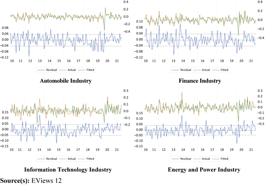
We see that the fitted values of returns of the automobile industry and finance industry are close to actual values. Further, in the information and technology industry, the fitted values are not very close to the actual values, which indicate that the fitting of the model for this particular industry is not very good. As far as the energy and power industry is concerned, the fitting is good compared to the IT industry but not good when compared with the automobile and finance industry. So, the models for the automobile and finance industry have very good fitting which shows the stability of coefficients, hence these two models are very stable. But the model for the IT industry is not stable as compared to its counterparts.
4.3 ARDL model F bound test results for the determination of long-run relationship between sentiment sub-indices and returns of different industries
We have analyzed our model for the determination of the long-term relationship between Indian stock market return and sentiment sub-indices using ARDL bound test (Peseran et al., 2001). If F-statistic is greater than the value of the upper bound, this shows there is cointegration. If the F-statistic is in between the value of the upper and lower bound, it shows that the result is inconclusive. If F-statistic is less than the value of the lower bound, this shows there is no cointegration.
According to the results given in Table 10, the calculated values of f-statistic (Wald test) are equal to 18.25029, 11.19280, 10.82308 and 36.01389 for Automobile, Finance, Information and Technology; and Energy a Power industries respectively. Results show a significant relationship among return and sentiment sub-indices with optimal delay.
F bound test results
| F-bounds test | Null hypothesis: No levels relationship | |||
|---|---|---|---|---|
| Test statistic | Value | Signif | I(0) | I(1) |
| K | 11 | Asymptotic: n = 1000 | ||
| F-statistic for Automobile Industry | 18.25029 | 10% | 1.76 | 2.77 |
| F-statistic for Finance Industry | 11.19280 | 5% | 1.98 | 3.04 |
| F-statistic for Information and Technology Industry | 10.82308 | 2.5% | 2.18 | 3.28 |
| F-statistic for Energy and Power Industry | 36.01389 | 1% | 2.41 | 3.61 |
Source(s): Authors' calculation in EViews 12
For the existence of convergence, it is necessary that F-statistic is more than the upper bound . Based on the test, the existence of the independent convergence vector between Indian stock market return and sentiment sub-indices was proven indicating that there is a long-run relationship among returns of different industries and sentiment sub-indices. Results are significant at all levels of significance (1%, 2.5%, 5% and 10%).
4.4 Error correction form for different industries
Now we run the error correction form test to check whether our model adjusts monotonically (See Table 11). The value of CointEq(−1) shows the speed with which the model adjusts itself in the short run. This value basically shows the speed of convergence. The value of CointEq(−1) should be negative and less than and equal to 1. If it is positive or more than 1, this means there are oscillations in the model convergence.
Error correction form
| Industry | Variable | Coefficient | Std. error | t-statistic | Prob |
|---|---|---|---|---|---|
| Automobile | CointEq(−1)* | −0.842548 | 0.052073 | −16.18015 | 0.0000 |
| Finance | CointEq(−1)* | −0.961915 | 0.075914 | −12.67118 | 0.0000 |
| Information and Technology | CointEq(−1)* | −0.845753 | 0.067642 | −12.50333 | 0.0000 |
| Energy and Power | CointEq(−1)* | −0.958078 | 0.042117 | −22.74781 | 0.0000 |
Note(s): *Significant at 5% Level
Source(s): Authors' calculation in EViews 12
In the case of the automobile industry, the value of CointEq(−1) is −0.842548 which means 84% of the disequilibrium corrects itself within a month. The full convergence takes place in approximately 1.2 months (1/0.842548). The duration for adjustment is very high. Also, the t-statistic is very large, i.e. −16.18015, which means that the coefficient is highly significant.
The value of CointEq(−1) is −0.961915 for the finance industry. This implies that the model corrects its previous period at a speed of convergence of 96.19% per month. This shows that the model will adjust itself at a very high speed. The t-statistic is very large, i.e. −12.67118, which means that the coefficient is highly significant.
For the information and technology industry, the value of CointEq(−1) is 0.845753 which is very good. The model is correcting its previous period at a speed of convergence of 84.58% per month. The model is adjusting itself with high speed. The t-statistic is very large, i.e. −12.50333, which means that the coefficient is highly significant.
The model for the energy and power industry has a CointEq(−1) value of 0.958078 which means the model is correcting its previous values at a speed of convergence of 95.58% per month. The model is adjusting back to the equilibrium state at a very high speed. Also, the value of the t-statistic is very large, i.e. −22.74781, which means that the coefficient is highly significant.
4.5 Breusch–Godfrey serial correlation Lagrange multiplier (LM) test
We also check our ARDL models of different industries for serial correlation through Breusch–Godfrey Lagrange Multiplier (LM) Test. A model should be free from serial correlations in order to be stable. The results are in Table 12.
Breusch–Godfrey serial correlation Lagrange multiplier (LM) test for different industries
| Industry | F-statistic | Prob. F(2,114) |
|---|---|---|
| Automobile | 0.306480 | 0.7366 |
| Finance | 0.844155 | 0.4326 |
| Information Technology | 0.096567 | 0.9080 |
| Energy and Power | 0.439354 | 0.6456 |
Source(s): Authors' own calculation
Results show that the null hypothesis of no serial correlation is accepted at a 5% level of significance in the case of all industries. Thus, our ARDL models for different industries are free from serial correlation which is a sign of good model fitting.
4.6 CUSUM stability diagnostic test
The CUSUM test is based on the cumulative sum of the recursive residuals. The test checks the stability/instability of a model by plotting the cumulative sum of parameters (beta values). If the cumulative sum goes outside the V-mask area between two critical lines, the parameters are said to be unstable. We have employed the CUSUM test to check for the stability/instability of different models. CUSUM test results are given in Figure 2.
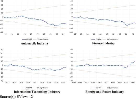
CUSUM stability test results show that ARDL models for different industries lie well within the 5% significance limits shown by the red lines and thus the models are stable.
4.7 Testing robustness of the model using ARCH heteroscedasticity test
We have checked our models for the robustness using Auto regressive conditional heteroscedasticity (ARCH) heteroscedasticity test. Heteroscedasticity is present when the standard deviations of a predicted variable, checked over different values of an independent variable are non-constant. The presence of heteroscedasticity in the model is a violation of one of the assumptions of linear regression modeling. Further, it affects the validity of econometric analysis and financial modeling. The null hypothesis for this test is— “There is Homoskedasticity in the Model”. The results are in Table 13.
Heteroscedasticity test results
| Industry | F-statistic | Prob. F(1,135) |
|---|---|---|
| Automobile | 0.011539 | 0.9146 |
| Finance | 0.567766 | 0.4525 |
| Information Technology | 0.102444 | 0.7494 |
| Energy and Power | 0.995509 | 0.3202 |
Source(s): Authors' calculation in EViews 12
Results indicate that the null hypothesis of homoscedasticity is accepted in all cases at a 5% level of significance. Thus, all 4 models are homoscedastic and free from heteroscedasticity and our models are valid.
5. Conclusion
The study contributes to examining the interesting issue of whether sentiment sub-indices influence the returns of select industries. By applying Auto Regressive Distributed Lag (ARDL) model on sentiment sub-indices and monthly industry return (S&P BSE 500) for the period from April 2010 to December 2021, we tested for long-run dynamic relationships also. The leading representative industrial indices have been used as a proxy for the industry return.
The sentiment sub-indices explain most of the returns of the automobile industry and explain the lowest of the returns of the information and technology industry. The negative Relationship of contemporaneous values of “Market and Economic Variable (PC1)” with the return of all industries is in line with Pandey and Sehgal (2019).
The insignificant relationship of current values of “Market Ratios (PC2)” (all industries) and the significant positive relationship of “Advance-Decline Ratio and High-Low Index (PC3)” with industry return (except information and technology industry) is in line with Brown and Cliff (2004), Dash and Mahakud (2013b), Kumari and Mahakud (2016) and Naik and Padhi (2016).
The negative relationship of “Price-to-Book Value Ratio and Liquidity in Economy (PC4)” with returns of all the industries supports the results of Sehgal et al. (2010).
In the case of “Oil Price and Industrial Production Index (PC5)” results are in line with Du, Gunderson, and Zhao (2016) and Naik and Padhi (2016). The negative coefficients of current values and lagged values of “Buy-Sell Imbalance and Foreign Direct Investment (PC8)” support the results of Naik and Padhi (2016) in the context of the automobile and IT industry. The negative coefficient of the “Trading-Volume Ratio (PC9)” supports the results of Kumari and Mahakud (2016) but in the context of the automobile and energy and power industry.
“Extra Return on Market Portfolio” and “Term-Spread” are two sentiment sub-indices (new proxies to the sentiment) that explain the returns of all the industries. To the best of our knowledge, no earlier studies have documented the impact of these two variables on the return of industries.
Thus, based on the results, the hypothesis of this study, indicating the long-run relation between sentiment and industry return, cannot be refuted. After the determination of the order of Vector autoregressive (VAR) based on Akaike information criterion, we have estimated the vector error correction model also. The obtained Error correction model (ECM) coefficients are close to 1 which shows that the speed of deviation adjustment from short-term to long-run is very high (1 month). Our models are robust in terms of coefficients, serial correlation and heteroscedasticity.
This study would be a valuable addition to the growing body of empirical literature on the relationship between sentiment and return in emerging stock markets like India. Findings are useful to policy-makers, regulators and the investors’ community. Policymakers and regulators should watch out for the impact of fluctuations in different sub-indices. Investors can search for the presence of exploitable arbitrage opportunities in Indian stock markets to earn above-normal returns on the basis of sentiment sub-indices but not on the basis of “Market Ratios” and “Put-Call Ratio”. Further, industries insensitive to the sentiment may be used for contrarian investment strategy exploration at the time of high sentiment. Mutual fund managers who wish to hedge against extremely volatile market behavior can use the non-sentiment-prone industries to protect the valuation of their funds.
The findings of the study are limited to the proxies used for investor sentiment. Some proxies may need to be either removed or added. Survey methods can also be used to expand the study.
In the future, a comparative study can be conducted to analyze the impact of sentiment on industries’ return over the pre-crisis period, crisis and post-crisis periods. Also, it will give an idea of whether the sentiment index works well in these situations. We also wish to measure the impact of sentiment on industry return in the context of foreign markets where the work on sentiment is still in its nascent stage.
Notes
Details of the proxies identified are in Appendix 1.
Results of Augmented Dickey Fuller (ADF) test and Phillips Perron (PP) test are given in Appendix 2.
Details of 11 sub-indices are given in Appendix 3.
Selected 23 proxies can be found in Appendix 2.
It may be argued that the ARDL model cannot be applied when the endogenous variable is stationary. It is worth mentioning here that the ARDL model can be applied to both variables whether I (0) or I (1). (Peseran et al. (2001) and Omar et al. (2015) for details)
Autoregressive distributed lag model equations for select industries are given in Appendix 4.
References
Appendix 1
Details of variables used as proxy to the investor sentiment
| Sr. No. | Variables/Symbols | Description | Source |
|---|---|---|---|
| 1 | MKTTURN | Market turnover (₹) (Number of Shares Traded in the Market/Outstanding Shares in the Market) | SEBI website |
| 2 | NUMTRADE | Number of trades | SEBI website |
| 3 | TRADEQTY | 30 days moving average of traded quantity of shares | SEBI website |
| 4 | TVR | Trading-volume ratio (the ratio of turnover ratio to standard deviation of the market returns for the particular month) | SEBI website |
| 5 | ADR | Ratio of number of advancing shares to number of declining shares | SEBI website |
| 6 | COMPTRAD | Proportion of number of companies traded to total number of companies listed | SEBI website |
| 7 | VIX | VIX™ (Volatility index) | NSE website |
| 8 | FPI | Foreign portfolio investment (₹) | CDSL website |
| 9 | PCR | Ratio of number of put options to number of call options | NSE website |
| 10 | PER | Price-earning ratio (Market price/Earning per share) | BSE website |
| 11 | PBR | Price-to-book value ratio (Market price/Book price) of SENSEX | BSE website |
| 12 | DIVYIELD | Dividend yield (Dividend distributed/Market price per share) of SENSEX | BSE website |
| 13 | BSI | Buy-sell imbalance ratio ((Buy orders – Sell Orders)/(Buy Orders + Sell Orders)) | SEBI website |
| 14 | FDI | Foreign direct investment (₹) | Department for Promotion of Industry and Internal Trade website |
| 15 | RTVOL | Retail trading volume (₹) | BSE website |
| 16 | HLI | High-low index (10 days simple moving average of the record high percentage indicator) | SEBI website |
| 17 | EQRATIO | Ratio of equity (₹) in the total issue (₹) (Equity Issues/(Equity Issues + Debt Issues)) | SEBI website |
| 18 | NIFPO | Number of IPOs and FPOs in a month | SEBI website |
| 19 | ECORPREM | Difference between market return and risk-free rate of return | BSE and RBI website |
| 20 | XRETMP | Difference between return on market portfolio and market return | BSE website |
| 21 | OILPRICE | Oil prices (₹) | indexmundi.com |
| 22 | BDEPMCAP | Ratio of bank deposit (₹) to market capitalization (₹) | BSE and SEBI website |
| 23 | EQMF | Net investment in equity by mutual fund companies (₹) | SEBI website |
| 24 | LIQECO | Liquidity in the economy as measured through M3 (₹) | RBI website |
| 25 | INFLAT | Inflation in the economy as measured through whole sales price index | RBI website |
| 26 | PLR | Level of interest rate as measured through prime lending rate | IMF website |
| 27 | TERMSPRE | Term-spread measured as difference between 364 days treasury bills and 91 days treasury bills | RBI website |
| 28 | IPI | Level of industrial production as measured through industrial production index | RBI website |
| 29 | SHORTINT | Short-term interest rate as measured through Short-term deposit interest rate | RBI website |
| 30 | EXRATE | Exchange rate of the Indian rupee (₹) to US dollar ($) | OFX website (previously known as OzForex) |
| 31 | FEXRES | Foreign exchange reserves of India (₹) | RBI website |
| 32 | GDP | Gross domestic product | CSO and RBI website |
Source(s): Appendices are authors' own
Results of ADF and PP Test
| Variables | Augmented Dicky Fuller test | Phillips–Perron test | ||
|---|---|---|---|---|
| Level | First difference | Level | First difference | |
| p-value | p-value | p-value | p-value | |
| ADR | 0 | 0 | 0 | 0.0001 |
| BDEPMCAP | 0.3362 | 0 | 0.4432 | 0 |
| BSI | 0 | 0 | 0 | 0.0001 |
| COMPTRAD | 0.1685 | 0 | 0.1739 | 0 |
| ECORPREM | 0 | 0 | 0 | 0.0001 |
| EQMF | 0 | 0 | 0.0001 | 0 |
| EQRATIO | 0 | 0 | 0 | 0.0001 |
| FDI | 0.7294 | 0 | 0 | 0.0001 |
| FPI | 0 | 0 | 0 | 0.0001 |
| HLI | 0.028 | 0.0001 | 0.0977 | 0 |
| IPI | 0.1145 | 0 | 0.0212 | 0.0001 |
| LIQECO | 0.9949 | 0 | 1 | 0 |
| MKTTURN | 0 | 0.4944 | 0.0125 | 0 |
| NIFPO | 0.2364 | 0.0005 | 0 | 0.0001 |
| NUMTRADE | 1 | 1 | 0.9664 | 0 |
| OILPRICE | 0.3015 | 0 | 0.3041 | 0 |
| PBR | 0.1902 | 0 | 0.1611 | 0 |
| PCR | 0 | 0 | 0 | 0.0001 |
| TERMSPRE | 0 | 0 | 0 | 0.0001 |
| TRADEQTY | 0.0265 | 0 | 0.0308 | 0 |
| TVR | 0.0161 | 0 | 0 | 0 |
| VIX | 0 | 0 | 0 | 0.0001 |
| XRETMP | 0 | 0 | 0 | 0.0001 |
Source(s): Appendices are authors' own
Sentiment sub-indices
| Principal components | Variables/Symbols | Name of the principal component |
|---|---|---|
| PC1 | COMPTRAD | Market and Economic Variables |
| VIX | ||
| FPI | ||
| ECORPREM | ||
| BDEPMCAP | ||
| EQMF | ||
| PC2 | MKTTURN | Market Ratios |
| NUMTRADE | ||
| TRADEQTY | ||
| PC3 | ADR | Advance-Decline Ratio and High-Low Index |
| HLI | ||
| PC4 | PBR | Price-to-Book Value Ratio and Liquidity in Economy |
| LIQECO | ||
| PC5 | OILPRICE | Oil Price and Industrial Production Index |
| IPI | ||
| PC6 | PCR | Put-Call Ratio |
| PC7 | EQRATIO | Ratio of Equity in Total Issues and Total Number of Issues |
| NIFPO | ||
| PC8 | BSI | Buy-Sell Imbalance and Foreign Direct Investment |
| FDI | ||
| PC9 | TVR | Trading-Volume Ratio |
| PC10 | XRETMP | Extra Return on Market Portfolio |
| PC11 | TERMSPRE | Term-Spread |
Source(s): Appendices are authors' own

