

Chapter 10: Differential Privacy in Energy Systems

-
Published:2025
10.1 Introduction
The electricity network is one of the two largest infrastructures mankind has ever built, the other being the telephone network (now the Internet), both came into being around 130 years ago. This vast electricity network comprises high-voltage transmission lines that span long distances, forming the backbone of electricity distribution, and lower-voltage distribution networks that deliver electricity over shorter distances to consumers. In the United States alone, the grid connects more than 23,000 generators to countless loads such as buildings, machinery, and appliances. As of 2019, these generators have a total nameplate capacity of 1.2 terawatts and produced approximately 4 trillion kilowatt-hours of electricity, with close to 60% generated from fossil fuels.
The evolution of this network into a “smart grid” has ushered in an era where electricity generation, distribution, and consumption are more efficient and responsive than ever before. Smart grids leverage advanced communication technologies and data analytics to balance supply and demand dynamically, integrate renewable energy sources, and empower consumers with real-time information. However, this increased reliance on data introduces significant privacy concerns. Detailed energy consumption data, if mishandled, can reveal sensitive information about individuals and businesses.
For example, consider smart meters installed in homes that record electricity usage at fine-grained intervals. While this data helps utility companies optimize grid operations and offer personalized services, it can also expose intimate details about a household’s daily routines. An unauthorized party accessing this data could determine when residents are away, what appliances they use, or even infer lifestyle habits. Such privacy breaches not only threaten individual security but also erode trust in smart grid technologies.
How can we protect privacy in such a complex infrastructure network? In this chapter, we explore the intersection of energy systems and privacy, focusing on how differential privacy can be applied to protect sensitive data used as input to complex optimization problems adopted in power systems operations. In particular, we focus on optimal power flow (OPF) problems, which are essential for determining the most efficient way to distribute electricity across a network, and how differential privacy can enable the release of useful data sets that protect sensitive load information at specific locations.
Overview of the Chapter
We begin by introducing the fundamentals of electric grid operation in Section 10.2), to set the stage for understanding the complexities and data requirements of modern power systems. Next, we review the privacy challenges inherent in energy systems (Section 10.3) and discuss how the proliferation of advanced metering infrastructure raises concerns about unintended information disclosure. We then provide a mathematical model of power grids, in Section 10.4, which is essential for formulating optimal power flow problems. In Section 10.5, we focus on private DC optimal power flow data sets. We discuss the application of differential privacy to the DC-OPF problem, examining how to balance the need for data utility with the requirement to protect sensitive load information. Finally, we provide some remarks on the current state of research and future directions in integrating differential privacy into energy systems (Section 10.6). Our goal is to highlight the potential of differential privacy to enable secure and efficient operation of smart grids, encouraging further exploration and application of these techniques in the energy sector.
10.2 Electric Grid Operation
An electricity network consists of high-voltage long-distance backbone networks, called transmission networks, that connect to many low-voltage short-distance networks, called distribution networks. Different parts of the grid have their own nominal voltages, and voltages at all points of the network must be stabilized to within a few percent of their nominal values at all times.
The challenge of grid operation is to match supply with demand without violating voltage and transmission line limits. Secure operation refers to the grid’s ability to withstand and survive disturbances. There are two main types of disturbances. The first type consists of generation and transmission outages. The second type is due to non-dispatchable and volatile generations and demands. Secure operation is achieved through analyzing credible contingencies offline that may lead to voltage or line limit violations, reserving capacities in advance when scheduling generations, monitoring system state in real time, and taking corrective actions when a contingency occurs. Traditionally, resources for control are mostly bulk generators and, occasionally, a small number of industrial loads. In the future, flexible loads will also be included at scale.
The control architecture consists of three mechanisms operating at different timescales, from seconds to tens of minutes to 24 hours. Rapid small random load or generation fluctuations are handled by generators that can increase or decrease their outputs quickly and continuously. They are equipped with their own governors with droop control and provide regulation services, usually under automatic generation control, and on a minute-by-minute basis. Slower fluctuations at a timescale up to a real-time dispatch period, e.g., 5-60 minutes, are handled by generation units connected to the grid and provide load-following services. While load-following patterns of customers are highly correlated and often predictable, e.g., because loads often depend heavily on weather, regulation patterns tend to be smaller, more rapid and random fluctuations with zero mean. Both regulation and load-following services require continuous actions by participating units but these actions are typically small or predictable. They have been sufficient for dealing with the second type of disturbances traditionally, though they may become inadequate as volatility increases in the future.
In contrast, the imbalance due to the outage of a bulk generator or a major transmission line that imports power can be large and unpredictable, and can threaten system stability. Disturbances of this type are handled by reserve services and are scheduled a day in advance. This is called unit commitment. When a generator fails and is disconnected, supply and demand become unbalanced and frequency starts to drop. The power imbalance must be made up by other generators or reduction in load, in addition, the system frequency must be restored to its nominal value. If generation reserve capacity is insufficient to meet demand, frequency will continue to drop which can disconnect other generators to protect them from damage, potentially leading to involuntary load shedding and even system collapse. When a transmission line or transformer is disconnected, power flows in the network will redistribute and line limits can be violated, potentially leading to cascading line outages.
Over the last century the operation of the transmission network has been largely centralized, open-loop, deterministic and worst-case preventive; demands are forecast, and generations are centrally scheduled based on the forecast. Typically an operating point of the network is chosen so that the network can survive the outage of any single generator or transmission unit. This strategy has performed extremely well, since aggregate loads are fairly predictable, generators are fully controllable (dispatchable), the grid is often over provisioned, and large outages are relatively rare.
10.2.1 Need Control Paradigm
We are, however, at a cusp of historic transformation, driven by sustainability, to become more distributed, dynamic, open and complex. Renewable sources such as wind and solar will continue to replace traditional bulk generators, greatly increasing generation uncertainty and reducing traditional control resources. Distributed energy resources, such as small-scale wind and solar generators, electric vehicles, smart buildings, small appliances, and smart electronics, will proliferate, many equipped with the ability to measure, compute, communicate and actuate in real time. Unlike the large majority of endpoints today that are merely passive loads, these distributed energy resources are active endpoints that can introduce large, frequent, and random fluctuations in supply, demand, voltage and frequency. Their connected intelligence, however, offers a new paradigm to manage the future grid based on real-time communication, computation, and control. The continual increase in generation and demand volatility makes it necessary to close the loop and actively control these distributed energy resources at scale based on timely data.
Data are being collected by distributed energy resources behind the meters as well as by high resolution and synchronized phasor measurement units that are being deployed inside the infrastructure. These different types of data may be collected by different organizations at different parts of the network. They can all be useful for real-time control of the future grid, provided a standardized platform for data sharing can be developed that provides right incentives and preserve necessary privacy. In addition to the physical control of the network, there is an energy market, i.e., a commodity market for incentivizing a competitive energy supply industry. Although we won’t go into much detail here, there are three types of short-run markets in practice, a day-ahead market, a real-time market, and an ancillary services market. They are typically operated by an independent system operator at timescales ranging from minutes to a day. Traditionally these markets transact electricity produced by generators to meet inelastic demand. It the future they will also trade demand response from flexible loads. Data privacy issues will clearly need to be introduced into a market platform when this becomes possible. The focus of this chapter will be on releasing data sets that contain sensitive load data, i.e., power demands across a network, such that optimal power flow problems (a key element in grid management that matches power demand with production).
10.2.2 Markets
There are three types of short-run markets in practice, a day-ahead market, a realtime market, and an ancillary services market. They are typically operated by an independent system operator at timescales ranging from minutes to a day. Traditionally these markets transact electricity produced by generators to meet inelastic demand. It the future they will also trade demand response from flexible loads.
Day-ahead Market
Bulk generators such as nuclear, coal and gas generators still generate the majority of electricity today, e.g., they generate approximately two thirds of electricity as of 2020 in the US. They often need a nontrivial amount of time and cost to start up and shut down, e.g., the startup time for a nuclear plant can be on the order of hours. This motivates the day-ahead market which usually closes 12–36 hours in advance of energy delivery and determines which generators will be online and their output levels for each hour or half hour over a 24-hour horizon. The day-ahead market also computes consumption schedules, electricity prices, as well as capacity reserves based on the production offers and demand bids submitted by market participants. This is the problem of unit commitment.
Real-time Market
A real-time market, also called a spot market or a balancing market, operates at a timescale of minutes, e.g., 5–15 minutes. It computes adjustment to generation and consumption levels as well as prices and reserves at delivery time as uncertainty in generation, consumption or network state is resolved. This is the problem of economic dispatch and discussed in Section 10.5.2.
Ancillary Services Market
Finally markets for ancillary services are emerging, driven by reliability requirements in the presence of increasing uncertainty due to renewable or distributed generations such as wind and solar power as well as increasing ability to coordinate flexible loads such as smart buildings, electric vehicles, and other appliances to provide energy services. These services include reserve capacities for generator or transmission contingencies, or demand response for frequency regulation. Reserve capacities may be spinning reserve where a generation unit that is online may generate at only 80% of its capacity with the unused capacity reserved for contingency operation. They may also be non-spinning reserve where a more expensive fast-acting unit remains offline but is ready to be turned on within minutes of a contingency.
10.3 Energy Systems and Privacy
In this section we provide a brief overview of the different application areas within energy networks that have been studied from a privacy perspective. In some areas, differential privacy has already been applied, in others, its potential use is clear. We end this section with an application of the classical Laplacian and exponential mechanisms of differential privacy (see Chapter 1 for a review on these mechanisms) implemented on real data taken from an electric vehicle charging network in Pasadena, California.
10.3.1 Overview
The new distributed and dynamic architecture of the power network, in combination with intelligent sensing and metering is frequently referred to as the smart grid. In contrast to the traditional power networks, information flow in a smart grid is bi-directional. Individual users (consumers) can actively manage their energy use, simultaneously, energy producers can more effectively reduce ceiling capacity and better control usage via smart pricing. Smart grids will also make it possible for consumers to become energy producers. However, to make this a reality, vast amounts of time-series data is required from participating entities, and with this come many security and privacy concerns [MM09; ZPAB13; HRC19]. Smart meters (devices that monitor home power usage and can be used to switch appliances on and off automatically) are an obvious focal point for privacy concerns. It has been well known since the early nineties that non-intrusive appliance load monitoring i.e., passive measurements at the point of a traditional energy meter, can be used to identify exactly which appliances are being use in a home, and when [Har92]. Likewise, smart meters can also be used to infer home occupancy states [AR13]. Differential privacy is clearly a methodology that has great potential to resolve some of these concerns. We refer the reader to the following papers to get a sense of how differential privacy is applied; [Zha+15; MMA11; ZJWL14; GFDK19; GGP17; EE17; BBA16].
Beyond smart metering, differential privacy is finding application in several areas related to power and energy. In particular; the cost of introducing “noise” into the system and it’s effect on pricing in energy markets is considered in [BKJB13]. Within the context of electricity and gas markets [FMV20] examines differential privacy into Stackelberg games. Private data sharing for better renewable energy forecasting is considered in [GBP21], and electric load forecasting in [Eib+18]. Unintended information disclosure is highlighted as a security issue for electric vehicle (EV) charging in [ADPK20]. In the next section we provide a simple case study of differential privacy applied to an EV charging station’s data set.
10.3.2 Numerical Example: Electrical Vehicle Charging
In this subsection, we are going to show two examples where classic mechanisms are applied to data collected from an electric vehicle (EV) charging system; specifically the Adaptive Charging Network (ACN) based at Caltech in Pasadena, California. ACN was first deployed on the Caltech campus in early 2016 and the system uses smart scheduling algorithms to charge EVs for both Caltech and non-Caltech users.
As of 2020, ACN includes 126 level-2 EV charging stations (EVSEs) and 5 DC fast chargers (DCFCs) across three Caltech garages [Lee+20]. ACN is also operated at NASA’s Jet Propulsion Laboratory (JPL) as well as at over 100 other sites across the US. The charging data, including user demand, parking time, delivered energy, etc., are collected for every charging session from the Caltech and JPL sites, and the data are published through the ACN Research Portal, available at ev.caltech.edu. Currently detailed information of over 60,000 charging sessions is available. We use this data as a toy example to demonstrate how classic mechanisms such as Laplace mechanism and exponential mechanism can be used to preserve differential privacy for different energy system applications.
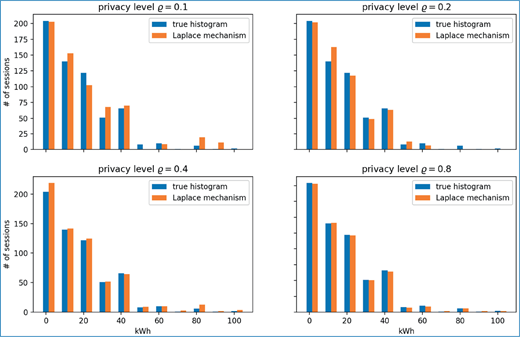
For this demonstration, we use the data from November 1st to November 30th, 2019 at the Caltech site. In the first example, we are interested in the distribution of user demand for each charging session. We set the query as the histogram of the user-requested energy (in kWh) for each session, and the ground-truth histogram is given in Figure 10.1 (blue bars). In November 2019, there were in total 611 charging sessions, and from the histogram we can see that though the highest singlesession demand was over 100 kWh, the majority of sessions requested less than 50 kWh. Roughly, 50kWh corresponds to a 200 mile driving range assuming the vehicle’s MPGe is around 136. Over half of the sessions requested less than 20 kWh.
To preserve differential privacy for a histogram query, a commonly used mechanism is the Laplace mechanism, which we will review in Section 10.5.2. Note that we use slightly non-standard notation and use ϱ-differential privacy instead of ε-differential privacy (c.f. Definition 10.2). The Laplace mechanism injects an additive term drawn from a Laplacian distribution to the ground-truth data. The variance of the distribution is chosen according to the query sensitivity and user-specified privacy level. The sensitivity of histogram query is 1, so the mechanism simply adds noise following Laplace distribution where ϱ is the desired privacy level. Figure 10.1 displays the mechanism output for ϱ = 0.1, 0.2, 0.4, 0.8. By Theorem 3.6 in [DR+14], the noisy histogram (orange bars) in each subplot in Figure 10.1 is guaranteed to preserve ϱ-differential privacy for the corresponding value of ϱ and can be released publicly. As the value of ϱ increases, the public histogram gets closer to the ground truth, and less privacy is preserved. On the other hand, the public histogram can still characterize the high-level statistical pattern of the private histogram. In this example, readers could easily learn from the public data that almost all the charging sessions in November 2019 requested less than 50 kWh and over half of them requested between 0 and 20 kWh.
Apply Laplace mechanism when the query is the histogram of requested kWh per session.
In the second example we focus on the categorical query. We want to know which day has the highest daily total demand (i.e., the summation of all the energy demanded during that day). Red bars in Figure 10.2 illustrates the total daily demand over the 30-day period. From the plot together with a 2019 calendar, we could easily see the weekly pattern that the demand is typically high during weekdays and drops over the weekend. Note that November 28th in 2019 is the Thanksgiving holiday, so the demand is also low on and after that day. Two days with the highest demand are Nov 8th and 12th, when the daily demands are as high as 771 kWh. As we query the date with the highest daily demand, we expect the mechanism to output Nov 8th or Nov 12th (or other dates with high demand) with high probability.
Application of the exponential mechanism to the query “what is the date with the highest load demand?”.
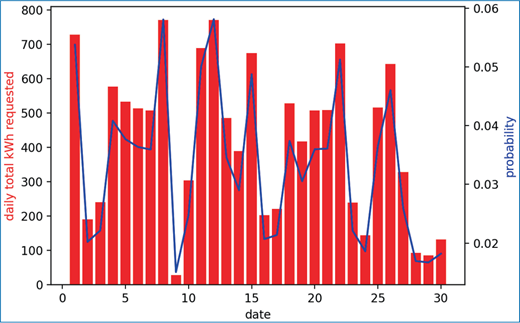
In this case, Laplace mechanism may not be an appropriate choice for two reasons. First, the Laplace mechanism always outputs floating point data, which makes no sense for categorical queries such as the date. Second, if we view the date as numerical data and compute its worst-case sensitivity, the sensitivity value could be larger than necessary. For example, it is possible that the date with the highest demand will change from Nov 1st to Nov 30th after we insert a new session record which increases the demand on Nov 30th, and it implies that the worst-case sensitivity is 29 if we view the date as numerical data. However, a more appropriate mechanism to process worst-case is the exponential mechanism. We refer to [DR+14; LLSY16] for the detailed derivation, and here we only present the high-level idea and illustrate the results on ACN data. To apply the exponential mechanism, we first choose a utility function u(d, o) where d is the dataset and o stands for the output (the date in our example). We let u(d, o) return the total daily demand on date o for dataset d, so we want the mechanism to return the date with large utility value. By the exponential mechanism, we output each candidate o with probability proportional to , i where Δu is the sensitivity of utility function u. The probability distribution to output each date has been shown in Figure 10.2 (blue curve). We can see that the probability distribution tracks the quality function well, so there is a fair chance for the mechanism to output the date with very high energy demand, though the true maximum may still be missed for privacy consideration.
10.4 Modelling a Power Grid
For the remainder of the chapter, we will narrow our focus from energy systems to power grids. In this section we will describe how to model power flow over a network. Of course, this is a vast topic that we cannot hope to cover in its entirety. Instead, we will focus on models that are suitable for formulating optimal power flow (OPF) optimizations. An OPF problem is a mathematical optimization problem, the solution of which determines how to distribute power over a network subject to physical an operational constraints. In subsequent sections of this chapter we will turn our attention to privacy preservation of data sets obtained from solutions to OPF problems. Our intention is to convey how tools from differential privacy can be applied in this setting, thus we have mostly opt for simplicity over realism. In many cases, the more realistic results don’t exist yet, in others, the realism simply clouds the results by introducing unnecessary notation and more equations.
10.4.1 Network Model
We begin by describing how the physical power network can be described mathematically. The starting point is to view a power network as a collection of nodes (where a node may correspond to a power source, sink, or both) end edges (transmission or distribution lines) which connect nodes. In power engineering, nodes are typically referred to buses. We will use the two interchangeably.
The most natural way to model such a system is via a graph where is the set of all buses in the network and denotes the set of edges connecting the buses. To reduce the notional overhead we will often omit the arguments and simply refer to a graph as . The set can be decomposed into two sets according to whether a bus is a power source (referred to as a generator bus, or simply a generator), i.e., a point at which power is produced and injected into a network, or, a power sink (referred to as a load bus, or simply a load), i.e., a point where power is consumed and removed from the network. The set can thus be decomposed as . In real networks it is common for a bus to consist of both generators and loads. Our representation does not preclude this, however, we will make the assumption that all buses in our networks are either generators or loads and not both. This assumption is not restrictive (in the DC power flow model) as we can always model a power system in this manner, it does however simplify notation and analysis. We denote the number of generator and load buses in the network by NG and NL respectively and denote N = NG + NL. For notational convenience, we assume the nodes are ordered as and . Buses are connected via the edge set , we label the edge set . When is undirected, if and only if . For directed graphs, if we say that l is the source and m is the target denoted by s(ei) = l and t(ei) = m respectively.
It will often be convenient to represent a via matrices. In particular the incidence matrix C ∈ ℝN×E describes how edges connect to vertices. When is undirected, a direction is arbitrarily assigned to each edge. The matrix C is then defined as
As we will see in subsequent sections, it will often be useful to overload our graph model to take into account weights on edges. These weights will be related to certain electrical properties of transmission and distribution lines. To accommodate this, we introduce a diagonal matrix W ∈ ℂE × E. Together with the incidence matrix, we can form the weighted N × N Laplacian matrix L = CWCT.
10.4.2 Power Flow Model
A power flow model provides a mathematical description of how quantities such as current, voltage, and power relate to each other at points over a network. Our goal here is to provide some intuition into how electrical engineers model these networks. The material covered is standard, some excellent references include [MLBB20; Bie15; Mom17]. However, the remainder of this chapter can still be understood purely from a mathematical perspective with no knowledge of the underlying physics needed!
In power engineering, we typically express such quantities as complex numbers. Consider a sinusoidal voltage function v(t) = Vmax cos(ωt + θV), using Euler’s identity we see that
where and denotes the real part of a complex number. Define the effective phasor, then the voltage function can be expressed as
Current and power can also be expressed as phasors in an analogous manner. The instantaneous power is defined as p(t) = v(t)i(t). Assume the voltage and current both have angular frequency ω, then the average power over the period is
It is not difficult to see that . However, this is only part of the story. Define the complex power as S = VI* and the reactive power where denotes the imaging part of a complex number, then
where superscript * denotes complex conjugation. When designing power systems, it is important to consider not just the average power P, but also reactive power, Q. For example, from the definition of S, it is clear that for fixed P and |V|, the magnitude of the current increases with |Q| to which there are associated thermal costs that should not be ignored. Finally, voltage and current are related to each other via I = YV, where Y is a complex number known as the admittance which we define as Y = G – jB (the reciprocal of admittance is impedance and is commonly denoted by Z, i.e., V = ZI). We are now ready to describe a model for how power flows over a network.
We begin by taking the graph that models the power network and labeling one of the buses as the slack bus for which we assume |V| = 1 and its phase is 0°. Without loss of generality we label the slack bus as bus 1. As we move to the network setting we will use bold-faced upper-case characters to denote vectors of voltages, currents, and power flow for the whole network.
Every transmission line (edge) in the network is modeled by the ⊓-model. Consider the line (j, k): In the ⊓-model, the line is described by the tuple of admittances corresponding the series admittance and two (not necessarily equal) shunt admittances at each end of the line, respectively. Note that there is only one series admittance for each line and so . Let Ijk denote the branch current from bus j (equivalently node j in ) to bus k (equivalently node ), and Ikj the current from bus k to j. The presence of the shunt elements means that summation of these two quantities is not necessarily zero. We now proceed to develop a set of equations that relates all the current injections I1, I2, … in the network to the voltages V1, V2, …. Collecting the quantities in a the complex vectors I and V and applying Kirchhoff’s current law at each bus in the network we have
where .
The complex N×N matrix Y is called the admittance matrix. Finally, combining the relationship between current and voltage through the network with complex power balance as defined by (10.1), we obtain
the net power injection at bus j. Including the slack bus, there are N equations in (10.2) in 2N complex variables Sj, Vj. The system of equations (10.2) can equivalently be written in polar form with 4N real variables Pj, Qj, |Vj|, and θj, where and Sj = Pj + jQj. To simplify notation, we denote and . When j = k (shunt admittances at bus j) we have that Gjj ≥ 0, Bjj ≤ 0, and for j ≠ k (line (j, k) series admittance), Gjj ≥ 0, Bjj ≥ 0. It follows that for each , (10.2) becomes
where θjk := θj – θk is the voltage phase angle difference for line .
Obtaining solutions to either (10.2) or (10.3) is known as a power flow problem. Typically, half the variables will be specified and the remaining variables must be solved for. The power flow equations are nonlinear and so iterative methods are often required to obtain solutions.
The reason for wanting to solve power flow problems in the first place is to determine how power will flow when parameters such as voltage requirements, generation demand and production are specified at each bus. Note that earlier we defined Sj to be the net complex power injection at bus j. The implication is that at each bus power may be produced and removed. So, formally , where superscripts g and d refer to generate and demand respectively. Buses in the network are typically classified as into three types; PV buses, PQ buses, and slack buses. This classification is somewhat synthetic, but useful for our purposes. Determining which variables in the problem are fixed, and which are specified, depends on the bus classification. See Table 10.1 for specific details. PV buses are typically generator buses, PQ buses are typically buses with a constant power load. The slack bus is required to ensure a solution exists and that power balance is achieved.
The focus of the remainder of this chapter is optimal power flow problems (OPFs). An OPF is an optimization problem where power flow equations (10.2) or (10.3) appear as constraints. In the next section we concentrate on a specific form of an OPF, and discuss where privacy issues arise and how differential privacy can be used to allow for the public release of OPF problem data.
Power flow equation data categorized by bus type.
| Data | Specified | Solve for |
|---|---|---|
| Bus type | ||
| PV | ||
| PQ | |Vj|, θj | |
| Slack | V1 = |V1| ∠0° | P1, Q1 |
10.5 Private DC Optimal Power Flow Data Sets
Optimal power flow problems seek to minimize (or maximize) a function, typically generation cost, user disutility, or power loss, subject to the physics of power flow (10.2), and network operational constraints such as line capacity, and voltage magnitude constraints. The OPF problem was first formulated by Carpentier in the 60’s [Car62] and it remains an active area of research today. OPF problems arise in many aspects of power engineering including unit commitment (determining which generators will participate in power production), economic dispatch (determine the power output of participating generators), N – K safety (ensuring network stability should K line failures occur), state estimation, and demand response, to name a few. The literature on OPF problems is vast and we will only cover OPF problem formulation at a very high level. For a detailed view of the OPF landscape we refer the reader to the following surveys [FSR12; HG91] and the tutorial [FR16].
10.5.1 Optimal Power Flow
Beyond their importance to power network operation, OPF problems receive so much attention because the power flow equations (10.2) are nonlinear (quadratic) functions. As such, the resulting optimization problems (in which the power flow equations are constraints) are quadratically constrained and non-convex. Such problems are NP-complete in general, and so heuristics are needed to provide solutions. Convex relaxations based on semidefinite programming is a popular approach for solving OPF problems, and in many cases such methods come with strong theoretical guarantees, see [Low14a; Low14b] for an overview of this type of approach and [Zoh+20] for general conic optimization formulations. We will now describe the most general form of an OPF problem and then restrict our attention to a more manageable special case.
We stack all complex powers injections into the vector S = P+jQ, an alternating current (AC) OPF problem takes the form:
where Pg is the vector of real power generation. Here we have assumed no shunt devices, i.e., for all j. The objective function f is quadratic and assumed to be separable across all generators. Generically, it takes the form:
The vectors Vmin and Vmax contain non-negative lower and upper limits for the squared voltage magnitudes. The voltage magnitude vector inequalities are taken element-wise. With slight abuse of notation, the constrains on S should be read as two sets of constraints, one on the real part and one on the imaginary part. The OPF formulation (10.4) is sufficiently general so as to allow:
Unbounded load or generation at bus .
Arbitrary slack bus values: , with corresponding net power injection unbounded.
Fixed net power injection: .
As mentioned above, solving (10.4) is theoretically and numerically challenging. Given that solving OPF problems in the general form of (10.4) is not straight forward, we will primarily work with a restricted version of (10.4) known as the DC-OPF, where DC stands for direct current. The DC-OPF model is convex (and hence global solutions can be found), furthermore it is formulated as a linear program (LP) which is perhaps the best understood convex programming class, and many efficient solvers exist allowing us to solve them at scale. With respect to differential privacy, the DC-OPF problem is more fully understood. We will describe work on privacy preserving mechanism for the full OPF problem towards the end of the end chapter.
10.5.2 DC Optimal Power Flow
We now turn our attention to DC OPF problems [SA74; PMVB05; CV14]. Although DC-OPF problems are more restrictive than their AC counterparts [OCS04], the simplicity of dealing with a linear program allows us to focus more on data privacy and less on the intricacies of non-convex optimization. The following assumptions bring about the DC power flow model (which then become constraints in an optimization problem):
Voltage angle differences across a line are assumed to be small. For a line , use the small angle approximation sin(θi – θj) ≈ θi – θj where angle are measured in radians.
Voltage magnitudes, |Vi| are assumed to be constants.
All lines are lossless, i.e. Gik = 0, and so Yik = jBik for all .
Under normal operating conditions, the voltage magnitude constants are approximately one. Applying the above three points to the expression for real power at bus j in (10.3) gives:
In the DC model, reactive power is ignored and so Pj completely characterizes the power flow. Of use to us is the fact that (10.5) is linear in the decision variables θj, θk, and Pj. As a consequence of (10.5) (equivalently, by definition of a lossless line) it follows that , i.e., active power is conserved across the network. Active power conservation does not hold when dealing with the AC power flow equations where the loss on a given line is proportional to the inverse of the magnitude of the line impedance multiplied by magnitude of the voltage difference squared. The final assumption made is to replace the quadratic cost function f in (10.4) with a linear cost function . Recalling the definition of the Laplacian matrix from Section 10.4.1, we arrive at the DC-OPF problem:
which is a linear program. The vector P ∈ ℝN is the vector of net power injections with each element assigned to be a generator or load. The subset that correspond to generators are denoted Pg. The matrix C is the graph incidence matrix, and B is a diagonal matrix containing the (positive) susceptances. The susceptances are obtained from the elements Bjk, i.e., the complex part of the admittance matrix.
Definition 10.1.We refer to the vectors, andpminas the network parameters and define the network parameter vector.
With a tractable model for power flow optimization in hand, we turn our attention to the issue of privacy. The natural questions to consider are; i) what data is it that needs to be kept private (we will also motivate this with the qualifier “and why”)? and, ii) is it possible to use differential privacy in this setting. The answer to part ii) should come as no surprise given the title of this monograph and the length of this chapter – yes, but with significant modifications. To answer the first question, we must consider the DC-OPF problem (10.6) (from now on referred to simply as the/an OPF problem) and note that it encodes the network model and the power flow equations. It may be surprising to many that it is the demand at the load buses that grid operators are most keen to keep private. Network topology can mostly be inferred by inspection (it’s difficult to hide above-ground power lines, power plants, and substations). Generation data is often publicly available (often in aggregate form) and the various constraint values need not often be known precisely. We thus focus on the problem of keeping load data private as we address the following three points:
The data that we would like to publicly release as (Pg, Pl). The net power at every bus in the network is Pi which we have decomposed into and for i = 1, … N. The main concern is that Pg is dependent upon Pd, specifically it is related through the deterministic optimization problem (10.6). This dependence needs to be accounted for, else information about Pl may be inferred from Pg (and the publicly available aggregate statistics for Pg).
The OPF (10.6) encodes the physical structure of the power network . A fundamental question here is how the network structure affects achievable privacy levels. Put another way, is the data generated by some power network “easier” to keep private simply because of the network topology? To what extent can this be quantified?
Similarly, how do the OPF constraints affect privacy guarantees?
At this point it is important to make two points. There exists a wide body of work on differential privacy and linear programming (and optimization more generally). The goal of this work is not to privately solve a linear program. Our goal is to be able to publicly release the data set (Pg, Pl) with a differential privacy guarantee along the lines of “changes in generation data will not disclose sensitive load data”. The second point we wish to make is that we are releasing the data so that data users can analyze the data and run their own OPF algorithms on. As such, we provide no guarantees that the the released data will be the solution to any OPF problem. We do not believe this to be restrictive as the OPF cost function and exact constraints are likely not available anyway. Users of the data will have accurate load demand data that (satisfies a differential privacy guarantee) to work with. Load data is typically the most important part of the data set – and most difficult to obtain. In later sections we describe work work where the data released does satisfy an AC optimal power flow problem.
Recalling that we assume the slack bus is bus 1, we also make explicit the partition on the Laplacian equality constraint;
and assume that (10.6) is well-posed, i.e. upper-bound constraints are greater than or equal to lower-bound constraints. For simplicity we focus on the Laplace mechanism which relies on the Laplace distribution . For a random variable , the probability density function is given by
the variance is given by σ2 = 2b2. Intuitively an increase in b corresponds to the distribution flattening out and spreading about the origin. For the purposes of establishing notation we now state some well known results that we will build from.
Suppose that is the data space for n users. A query is a function . In many cases, statistical queries correspond to r = 1. A mechanism, , is a randomized function of . In this work we shall consider additive mechanisms of the form where Y is an appropriately defined vector of random variables.
Definition 10.2 (ϱ-Differential privacy). The mechanismpreserves ϱ-differential privacy if and only if for allsuch that ||d – d′||0 ≤ 1 and all, we have
An intuitive way to understand this definition is to rearrange it and use the approximation exp(ϱ) ≈ 1 + ϱ for small positive ϱ, thus
From this we see that when d and d′ differ by a single element, the probability density of the corresponding mechanisms are similar. The similarity is characterized by q which is referred to as the the privacy budget.
Theorem 10.3 (Differentially private Laplace mechanism). The Laplace mechanismwithfor i = 1, …, r, where
provides ϱ-differential privacy.
The non-negative scalar Δ is the ℓ1 sensitivity of the query . Theorem 10.3 clearly shows us that the variance of the distribution depends on the sensitivity of the query and the level of privacy required. The more sensitive a query is, the “more” noise that must be added to attain a fixed privacy level. Similarly, when less privacy is required, the variance of the distribution decreases.
In the case of optimal power flow data, d = (Pg⋆, Pl). To emphasize the relationship between the load demand and power generation, we introduce the “OPF operator”. Informally, the OPF operator is a nonlinear operator that maps the vector of power loads Pl, solves an OPF problem, and returns the optimal vectorii of power generation Pg⋆. We express this operation as . From this point on, we drop the * from our notation. It should be implicitly understood that returns an optimal solution. It will also always be clear from context which OPF problem is being solved. Using this notation, we can now express the problem data as , which leads to the ℓ1 sensitivity function
which because of the complex dependencies between load and optimal generation, is a significantly more complicated object than (10.7). Indeed, characterizing the sensitivity function (10.8) is the central to developing an understanding of how differential privacy can be applied to optimal power flow data. As “defined” so far, the OPF operator is applicable to both AC and DC OPF problems. However, at the time of writing, little is known about the behavior of when the associated OPF problem is anything other than a DC problem. It is also important to note that is specific to the way the an OPF problem is modeled. In the AC setting, the same power flows can be modeled in different (but equivalent) ways which leads to different OPF problems – the AC OPF Problem 10.4 is just one realization, a different realization will induce a different . We will now focus out attention on the DC OPF operator.
10.5.3 The DC OPF Operator
The OPF operator has been studied in detail in [ZAL20; AZL20] in the DC setting. In this section we will provide a summary of the key results regarding the sensitivity function. In subsequent sections these results will be leveraged to help us understand how network structure and OPF problem data (constraint limits, cost function) determine variance of Laplace distribution required to provide ϱ-differential privacy guarantees.
The first issue we address is when does return a unique solution? Even although (10.6) is a linear program with a polyhedral constraint set, there is no guarantee that there is a unique solution. In this case will return the set of all optimal generation vectors. Working with set-valued operators is not trivial and we would like to avoid such a situation. Fortunately, this is straight forward. In [ZAL20] the precise conditions for uniqueness of solution were provided. The exact conditions are somewhat involved and would require several new sets to be defined, which for this chapter would clutter the presentation. Instead, we shall use the fact that the necessary sets are dense with respect to larger, easy to specify sets. The consequence of this is that should the specific problem instance under study fail to meet these conditions, then with probability one, a perturbation to the problem description will satisfy the criteria. For this reason we make the following assumptions:
Assumption 10.4.The OPF operator maps to a singleton, i.e., . The mapping is continuous everywhere and differentiable almost everywhere. Furthermore, all points in the image space ofare optimal solutions of(10.6).
Remark 10.5.Loosely speaking, the assumptions above are valid when the coefficientscifor i = 1, …, NGare all non-negative. The parameters that define OPF(10.6), , are chosen such that a feasible solution exists, and the feasible solution has NG – 1 active inequalities. Full details are available in [ZAL20].
The OPF operator is now used to define the concept of “monotonicity” for power networks. Recall that a function f : ℝn → ℝ is said to be monotonic (sometimes referred to as “order preserving”), if for all x, y ∈ ℝn we have that
where the inequality on the left hand side is taken element-wise. In order to reconcile monotonicity with differential privacy, we will consider the case where f above is replaced by and x and y are constrained to differ in exactly one element.
Definition 10.6 (Monotonicity). A power system is said to be monotone if for allsuch thatx ≥ yand withxandybeing feasible load profiles, we have that.
In words, a power system is monotone if, given a vector of power demands (loads) and corresponding optimal generations, a load increase will not cause a decrease in power generated at any bus in the network.
Monotonicity, as per Definition 10.6 attempts to characterize how the optimal power generation reacts to a change in load. Clearly, monotonicity is related to the ℓ1 sensitivity function (10.8). Unfortunately, Definition 10.6 only provides a partial characterization of the load–generation relationship. In order to provide a complete characterization, we introduce the the notion of (δ, ε)-monotonicity.
Definition 10.7 ((δ, ε)-monotonicity). For δ > 0, and ε ≥ 0, a power system is said to be (δ, ε)-monotone if for allsuch thaty + δ1 ≥ x ≥ yand ||x – y||0 = 1, we have that
where for [z]– := min{0, z} for z ∈ ℝ.
In the definition above, the parameter ε covers for the fact that power generation is allowed to decrease, and δ describes the “spread” of the load y. Clearly, any system which is monotone according to Definition 10.6 is (δ, 0)-monotone for any choice of positive δ. Note that any value of ε that satisfies the inequality in Definition 10.7 is valid, however, when we make use of monotonicity in the context of privacy later on, the smaller ε is, the better. Determining the (δ, ε) parameters is in general a difficult task. For certain classes of networks we can provide analytic expressions.
IEEE 9-bus Network
We first consider a simple test network with 9 buses. The network consists of 3 generator and 6 load buses. The IEEE 9-bus network is perhaps the simplest and most commonly used network for studying optimal power flow problems. Here we use it to illustrate the fact that monotonicity can be too stringent a requirement for even simple networks. We then use it to provide some intuition about (δ, ε)-monotonicity. The network is depicted in Figure 10.3. At each of the generator buses and two of the load buses, we have included a graph which shows how various loads and generations change.
We first consider bus 9 (lower left corner of Figure 10.3). The graph associated with bus 9 shows that the load, i.e., power demanded at this bus increases with time. It is assumed that all other loads remain constant. Note that although the line looks continuous, in reality this is a set of discrete loads. For every value of the load, we solve (10.6), or equivalently calculate and plot the resulting generations for each of the three generators on their respective graphs. If the network (for this particular choice of network parameters) was monotone, then graphs at each of the 3 generator buses would all be non-decreasing. At bus 1, the graph is non-decreasing. In fact, it is constant. This is likely because the generator is at its maximum capacity. At bus 3, an increase in power generation is observed. Surprisingly, at bus 2, the generator decreases its power output. From this we conclude that the system in not monotonic. This simulation highlights the complexity optimal power flow problems – despite bus 2 being closer to bus 9 (in a graph theoretical distance sense) it is bus 3 that provides the additional power required. In Figure 10.3 we also consider the case where the load at bus 5 is varied (with all other loads kept constant) and see similar results (dashed lines). We state the following theorem without proof.
IEEE 9-bus network. The ‘G’ nodes denote generators, and the numbered lines are transmission lines.
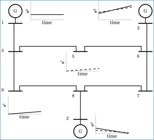
Remark 10.8.The IEEE 9-bus network is (δ, 2.01δ)-monotone. This parameterization is invariant to changes in the cost function and ξ.
The implication of this is that the optimal generation at any bus in the network will not decrease by more than 2.01 times the increase in the load.
In addition to monotonicity, we will also discuss derivatives of . Combined with monotonicity, this will provide an almost complete understanding of the sensitivity of the problem. As with monotonicity, the exact details for when derivatives can be taken are described in [ZAL20]. For now we rely on Assumption 10.4 and assume everything is well defined. Of interest to us is the how the optimal power generation at each generator changes as a function of changes in the load. We denote the vector of derivatives of with respect to the loads by .
Theorem 10.9.When Assumption 10.4 holds, the local derivativeexists and the set of binding constraints in(10.6)remains unchanged.
The second part of the statement in Theorem 10.9 is useful because it also tells us about the behavior of the optimal power flow problem. It tells us that for almost all the problem instances, when the load changes, any constraints that have hit their upper or lower limits will remain at those limits and no new constraints will reach capacity. We can actually go one stage further and write down an explicit algebraic relationship between the load and the optimal generation and voltage angle. To proceed, we need to define two sets that account for binding inequalities in (10.6).
Definition 10.10.Consider the DC OPF problem(10.6)and the graphassociated with it. Assume that(10.6)has been solved. Define the setas the set of generators producing power at maximum or minimum capacity, i.e., equal to the corresponding value inor. Likewise do the same for edges with power flows at maximum or minimum capacity corresponding topmax, pmin. Denote this set as.
We will not prove this here, but it can be shown that the total number of active constraints is
where |·| applied to a set denotes cardinality.
The Jacobian matrix defines the effect of all load changes on all optimal generations. Assume the network parameters are fixed, i.e., ξ is constant and that the coefficients in the cost function ci are all positive. Formally, the Jacobian is
However, if one has access to the solution of (10.6) then the Jacobian can be stated explicitly as a function of ξ and . We briefly introduce the following notation; let IN denote the n × n identity matrix. Given a set let denotes the matrix formed by stacking the rows of IN indexed by the elements of .
Theorem 10.11.When Assumption 10.4 holds, and the set of binding constraints of(10.6)is known, the JacobianJ(Pl ; c, ξ) can be explicitly written as
where, whereL = CBCT, and
and the inverse always exists.
The Jacobian matrix is useful in its own right, it also serves two other purposes. It can be used to provide an upper-bound on the ℓ1 sensitivity Δ – although we won’t pursue that further here. The Jacobian also provides useful insight into how to gauge the (δ, ε)-monotonicity parameters.
Taken together, Definitions 10.7, 10.10, and Theorem 10.11 provide all the information about the sensitivity of required in order to apply differential privacy to the data set d =(Pg⋆, Pl). For details on how to compute sensitivity, the reader is referred to [ZAL20; AZL20]. Note that the Jacobian definition and the closed-form expression produce the same matrix. Unless a specific form the Jacobian is required, we drop the arguments and simply refer to it as J.
10.5.4 Differential Privacy
We are now in a position to integrate the results from the previous section regarding sensitivity, with the classical ideas of differential privacy. For simplicity, we focus on the Laplacian mechanism. We make no claim about this mechanism being “perfect” for power system data sets. The goal is to demonstrate that potential for privacy methods in this application domain. Proofs of the main results can be found in [ZAL19]
To reiterate, our goal is to release data sets of the form d = (Pg⋆, Pl) in order for users to i) run statistical queries on the load-demand data, and/or ii) solve optimal power flow problems using realistic load data. With regards to the second problem, network parameters ξ, and the cost function may, or may not, be publicly available. We assume that the network graph is available.
The mechanism acts on both vectors Pg⋆ and Pl, for brevity, instead of writing , we will instead simply write and it is to be implicitly understood that the optimal generations are obtained by solving an appropriate DC optimal power flow problem.
We will now show that the task of designing a mechanism that hides individual load changes, follows the classical results closely. Indeed, most of the difficulty was in formulating how to measure query sensitivity when the query involves solving a linear program. The first step is to modify the definition of differential privacy.
Definition 10.12 (Δ, ϱ-differential privacy).For Δ > 0 and ϱ > 0, the mechanismis said to preserve (Δ, ϱ)-differential privacy if and only if for all (Pl)′ and (Pl)″ such that
and for all, we have
Remark 10.13.The notation used in Definition 10.12 should not be confused with the standard notion of (ε, δ)-differential privacy used outside of this chapter. We also reiterate thatis shorthand for.
A straight forward application of Theorem 10.3 can be applied to Definition 10.12.
Lemma 10.14.Assumeis a deterministic query. The mechanismwithfor i = 1, …, r, preserves (Δ, ϱ)-differential privacy, if for any (Pl)′ and (Pl)″ such that ||Pl)′ – Pl)″||0 ≤ 1 and ||Pl)′ – Pl)″||1 ≤ Δ, Δ1satisfies.
This result doesn’t transparently take into account the underlying properties of the network or the associated OPF problem. Before we present the most general and transparent result, we require one final definition. Denote by the Jacobian matrix of the query function, i.e., the matrix of partial derivatives of the query with respect to changes in the load vector.
Theorem 10.15.Suppose a power system is (Δ, ε)-monotone, andthe magnitude of all the elements in the Jacobian matrixare upper bounded by τ. Then the mechanism, with, provides (Δ, ϱ)-differential privacy.
The theorem above makes it clear power system with associated optimal power problems that are far from monotone (large values of ε) require distributions with a significantly larger variance than their monotone counterparts. Note that Theorem 10.15 is only applicable for smooth and differential queries, and the Jacobian matrix is different from the Jacobian matrix J of operator, which we defined earlier. One way to interpret Theorem 10.15 is that the query can be viewed as the composition of functions and . By the chain rule, its ℓ1 sensitivity can also be decomposed as the sensitivity of (characterized by τ) and the sensitivity of (characterized by (Δ, ε)-monotonicity).
Corollary 10.16.Let τ andbe defined as in Theorem 10.15. A monotone power system with, ensures (Δ, ϱ)-differential privacy.
One has to be careful when interpreting the Corollary 10.16. As any monotone system is (Δ, 0)-monotone for any value of Δ > 0, it is tempting to simply make Δ arbitrarily small in order to make arbitrarily small. However, Δ controls the privacy level as well, thus making it arbitrarily small will compromise more privacy of the power system data.
The final scenario we consider concerns aggregated data. It is often the case that power flow data is available in aggregate form. Most often, data from a geographical region is pooled, and summary statistics about the data set are released. We consider the following simple scenario (more complicated settings are easily accommodated for): Instead of the data owner releasing d(Pg⋆, Pl), summary statistics for certain “regions” are released. A disaggregation algorithm then acts on this data to try and reverse engineer the original d(Pg⋆, Pl). Of course, exact recovery is almost surely impossible, but generating estimates of the data that is consistent with the aggregated data is possible [AZL18]. Let’s make things more concrete. Assume the power network and data set we care about has been split into m distinct regions , where . For simplicity assume that for all i, j. The aggregation query for region i returns two quantities, the sum of the load and the sum of the generation:
where again we have dropped the ⋆ superscript from the generation vector. The data owner discloses corrupted versions of and . we assume that these statistics are to be released using the Laplacian mechanism. In a more realistic scenario, the exponential mechanism would be used as this may prevent sign changes in the data. We pursue the Laplacian mechanism as it fits with the results presented so far. The Laplace mechanism adds iid Laplace random variables and is defined to be
with and . Using this definition of the aggregation mechanism we arrive at the following result:
Lemma 10.17.Let the power system of interest be (Δ, ε)-monotone. The mechanismpreserves (Δ, ϱ)-differential privacy whenfor i = 1, …, m are i.i.d. random variables drawn from.
An important observation to make is that the variance of the Laplace distribution in Lemma 10.17 does not depend on the number of aggregated regions m, or the number of buses in a region. For the aggregation query, it is straight forward to show that the upper bound, τ in Theorem 10.15 is equal to one.
10.5.5 Beyond DC-OPF
The previous section outlined how differential privacy can be applied to data generated from DC OPF problems. There is however a body of work that applies differential privacy to OPF problems with the full AC power flow equations in various privacy scenarios: [FV18; MFV20b; MFV20a; Dvo+20]. We won’t delve deeply into this topic, however we will illustrate the difficulties of dealing with AC optimal power flow problems and describe how the work in [MFV20a] addresses these problems.
The fundamental issue that arises when dealing with the AC-OPF Problem 10.4 and its variants, is that perturbations to the load profile may result in an infeasible optimization problem. Moreover, even when the perturbed problem is feasible, the magnitude of the difference between the true optimal solution and the perturbed solution may be large. The closeness of the two solutions is termed fidelity. In the DC setting, fidelity is quantified using the results characterizing the sensitivity of the operator as described in Section 10.5.3. Unfortunately, there is no straight forward extension to the AC-OPF setting. However, the abstraction of as a mapping from load to optimal generation is useful and used without the theoretical guarantees provided in the DC setting. In [MFV20a], algorithms are developed with two goals in mind:
Privacy: The vector of (complex) demands Sd and the perturbed loads should satisfy:
and for all j ≠ i, where α > 0.
- For Sd and satisfying the adjacency relationship above,
- Fidelity: The obfuscated loads provide an objective value that is close to ground truth:for β > 0, where ) with f the cost function from (10.4). Note, here we have overloaded to return a solution to an AC optimal power flow problem. No claims about uniqueness are made. When multiple optimal solutions exist, a single solution is chosen at random.
Here we highlight some of the subtleties and difficulties of dealing with AC power flow models. The first obstacle in out path is that the Laplacian mechanism now needs to be applied to a query which may return complex values. Inspired by the work from differential locational privacy [ABCP13], complex numbers are represented in a polar coordinate system (as opposed to a planar system) and the polar Laplacian distribution is used. A desirable property of the polar Laplacian pdf is that the the radius and angle (that define the random complex variable) can be drawn independently from each other. In contrast, using a multi-dimensional Laplacian distribution would require drawing both parameters together in order to achieve the correct scaling. As a result, drawing the random variable z = r exp(jθ) is done by drawing θ uniformly at random from [0, 2π). Obtaining r is a two step process: first, draw a scalar p uniformly at random from [0, 1) and the set ), where
and W–1 is the (-1 branch of the) Lambert W function. The ε term is the measure of differential privacy required in the classical sense of ε-differential privacy. The output of the privacy stage is a load vector that is additively corrupted by random variables from the polar Laplacian distribution. This intermediate vector will be the input to the fidelity phase.
The fidelity phase is more challenging. One way to view this phase is as postprocessing the complex vector . Formally it takes the form of a bi-level (sometimes referred to as a multi-stage) optimization problem [Dem02]:
We re-iterate that here in notationally overloaded and it refers to a mapping of complex load demands to optimal complex power generations through the AC-OPF Problem 10.4. The interpretation of the fidelity post-processing stage is that of re-distributing the Laplacian noise that was introduced in the first step of the process. While the combination of the polar Laplacian distribution and the bi-level post-processing stage achieve the two goals set out at the beginning of the section, unfortunately, solving (10.9) is intractable. Indeed, bi-level programs are strongly NP-hard, moreover, verifying a solution of a such a problem is NP-hard [VSJ94]. The work in [MFV20a] proposes three relaxations to the fidelity stage, each of which satisfies the bound
where is the is the output of (10.9). Extensive numerical simulations assess the accuracy and typical behaviors of the three relaxations in addition to their computational run-times. It is shown that the methods proposed offer orders of magnitude better accuracy than naively applying the Laplacian mechanism to the load data.
10.6 Concluding Remarks
In this chapter we have provided a high level overview of modern energy systems, with a focus on the path from energy production to transmission and control. Our aim was to highlight the need for privacy in energy systems, and specifically examine how differential privacy can be applied in relation to optimal power flow data. The majority of the chapter examined the DC-OPF setting where convex (linear) programming is the algorithmic tool of choice. We concluded by dipping into the significantly harder problem of preserving privacy of AC-OPF data, where we tried to highlight some of the inherent challenges.
This is a new and rapidly evolving area of research, we hope this survey will attract more attention to research at the interface of energy and privacy.
Here we use the fact that the utility function is monotone with respect to o. In a more general setting, the probability should be proportional to .
Here we assume that the optimal solution is unique, and this assumption will be further discussed in the next subsection.
