

We used difference-in-differences research design to investigate the effect of the outbreak of extreme environmental events near firms’ headquarters on the cost of debt.
Using a sample of Chinese firms listed on the Shanghai and Shenzhen A-Share markets from 2004 to 2020, we find that treated firms, those that have extreme environmental events occurring within 25 kilometers of their headquarters, have a higher cost of debt.
We find an increase in the cost of debt for firms headquartered in areas where local environmental events occur, suggesting that the outbreak of extreme environmental events strengthens local government’s environmental enforcement and supervision.
Our paper contributes to the emerging literature on the role of environmental risk and performance in the context of debt financing. We extend prior literature on the determinants of the cost of debt from the perspective of the exogenous extreme environmental events.
1. Introduction
In emerging economies, where poor legal and institutional environment have hindered firms from acquiring funding from other sources, such as the equity market, debt financing is the primary means of financing [1]. Therefore, understanding the factors that affect the cost of debt for firms is both significant and economically important. Given that environmental issues have gradually attracted the attention of government, firms, academia, media and the general public, a significant body of academic research has focused on the impact that corporate environmental risk or performance has on the cost of debt (e.g. Thompson & Cowton, 2004; Sharfman & Fernando, 2008; Schneider, 2011; Jung, Herbohn, & Clarkson, 2018; Eichholtz, Holtermans, Kok, & Yönder, 2019; Chen, Hasan, Lin, & Nguyen, 2021).
Thompson and Cowton (2004) found that banks evaluate their environmental risks based on a firm’s environmental protection status. Prior studies (Jung et al., 2018; Herbohn, Gao, & Clarkson, 2019; Chen et al., 2021) have documented that the cost of debt is higher for firms with higher levels of chemical release or exposed to carbon-related risk. Sharfman and Fernando (2008) document that a high level of environmental risk management contributes to corporate debt financing. Clarkson, Li, Richardson, and Vasvari (2008) provide evidence that debtholders exert pressure on firms to disclose environmental-related issues to assess potential liabilities in the future. While the evidence from prior research is directionally consistent, there are still questions regarding identifying the causal influence of environmental risk on the cost of debt. The relationship between environmental risk and the cost of debt can be biased by the omitted variables or reverse causality concerns. In this paper, we shed light on this critical topic using novel and exogenous incident-level environment emergency data and examine how exogenous environmental risk affects firms’ cost of debt.
Firms exposed to extreme local environmental events may incur higher debt costs through the regulatory and operational risk channels. First, the outbreak of extreme environmental events could lead to tighter local environmental policy and enforcement, which could result in high compliance costs for firms operating in areas subject to local extreme environmental events (regulatory risk channel). Extreme environmental events may raise public concerns and pessimistic environmental expectations, potentially prompting local government regulators to enforce stricter environmental regulatory requirements and industry standards and impose severe punishments for environmental violations (Pu et al., 2019). Thus, extreme environmental events expose firms to higher risks, which raises credit risk due to the increasing pressure of regulatory supervision on the environment (Weber, 2012). Fang, Liu, and Gao (2019) found that the Chinese environmental information disclosure policy tightens the restrictions on corporate financing. Considering the rise in public awareness and governmental oversight caused by the outbreak of extreme environmental events, lenders are also more likely to assess environmental risk when they make their lending decisions and charge higher interest rates. For example, numerous studies, including Thompson (1998), Coulson and Monks (1999), Thompson and Cowton (2004), and Weber (2012), have consistently demonstrated a positive correlation between developments in environmental legislation and the growing integration of environmental issues into lenders’ lending activities. These studies shed light on the significant impact that environmental regulations have had on shaping the behavior of financial institutions. In addition, sterner environmental enforcement and legislation could undermine firm’s revenues. Under an even worse situation, a firm might be forced out of business if it cannot afford to meet the compliance costs of increasing environmental enforcement.
Second, extreme environmental events can amplify the operating risk faced by firms, leading to detrimental effects on their operations. This is known as the operating risk channel. Extreme environmental occurrences near a firm’s operations can disrupt production processes and result in negative impacts on firm value and stock prices (Hill & Schneeweis, 1983; Klassen & McLaughlin, 1996; Graff et al., 2012; Krueger, Sautner, & Starks, 2020). These interruptions increase the likelihood of default by introducing uncertainty into firms’ current and future cash flows.
However, it is still possible that local extreme environmental events increase firms’ awareness of environmental risk management, reducing the uncertainty of future cash flows. Fines or negative media coverage of extreme environmental events alter the behavior of those responsible firms or institutions and the consciousness and actions of other firms that want to evade costly negative publicity and fines. For example, Chu, Liu, and Tian (2021) find that firms reallocate important financial resources and enhance both environmental innovation input and output in response to environmental spills occurring near their headquarters. Subramaniam, Wahyuni, Cooper, Leung, and Wines (2015) document that firms’ carbon risk awareness can motivate them to reduce their environmental risk exposure. Jung et al. (2018) also find that the adverse impact of firms’ historical carbon emissions on the cost of borrowing is lessened by the awareness of carbon risk. Thus, the empirical question of how the outbreak of extreme environmental events affects the cost of debt remains.
Following the literature (e.g. Pittman & Fortin, 2004; Minnis, 2011; Liu, Cullinan, Zhang, & Wang, 2016), we use a difference-in-differences research design to investigate the effect of the outbreak of extreme environmental events near firms’ headquarters on the cost of debt. Using a sample of Chinese firms listed on the Shanghai and Shenzhen A-Share markets from 2004 to 2020, we find that treated firms, those that have extreme environmental events occurring within 25 kilometers of their headquarters, have a higher cost of debt. The effect of the outbreak of extreme environmental events on the cost of debt is also economically significant. Specifically, we find that relative to the control firms, the treatment firms experienced a 0.029 increase in the cost of debt after the outbreak of local environmental events. This result is consistent with our argument that extreme environmental events could trigger stricter local environmental enforcement and monitoring, which could result in a higher cost of debt.
We conducted parallel trend tests to mitigate the concern that the documented results could be driven by pre-existing differences between areas with and without extreme environmental events. We find no pre-existing trends, as the treatment firms have significantly higher debt costs only after, but not before, the outbreak of extreme environmental events. This result indicates that the parallel trend assumption behind the DID model holds for our setting. We further perform a series of robustness checks, which include alternative measures of extreme environmental events, alternative definitions of debt cost and alternative window periods. Our results still hold.
Next, we explore the possible channels that link the outbreak of extreme environmental events to the cost of debt. First, we examine whether the outbreak of extreme environmental events indeed increases local environmental enforcement and monitoring, as captured by the proportion of words related to the environment in the government work report. We find that the outbreak of extreme environmental events increases the proportion of words that reflect the importance that the local government attaches to the environment and that reflect the environmental protection actions of the local government. Second, we investigate whether the outbreak of extreme environmental events increases the operational risk of firms, which in turn increases the cost of debt. We find that the outbreak of extreme environmental events does not significantly increase the operating risk of the treatment firms. In sum, our channel tests indicate that the outbreak of extreme environmental events increases the cost of debt through increased environmental enforcement and local government monitoring.
We further explore the cross-sectional variation in the relationship between the outbreak of extreme environmental events and the cost of debt. First, we examine whether the extent and severity of the extreme environmental events affect the relationship between the outbreak of extreme environmental events and the cost of debt. We find that the outbreak of more severe extreme environmental events leads to a higher cost of debt than the outbreak of moderate environmental events. Second, we examine whether the adverse effect of extreme environmental events on the cost of debt is weakened when the treatment firms can behave actively in response to environmental policy or protection. We find that the adverse effect of extreme environmental events on the cost of debt is weakened for firms that disclose environmental information, firms that receive awards for environmental protection, firms that disclose the emergency response mechanism for major environment-related emergencies, and firms that have higher ESG rating scores in the environment dimension. Third, we investigate whether firms’ relationship with the government can moderate the relationship between the outbreak of extreme environmental events and the cost of debt. We find that the effect of extreme environmental events on the cost of debt is weaker for SOEs and larger firms.
Finally, we examine the economic consequences caused by the outbreak of extreme environmental events and the increased cost of debt. First, we find that treatment firms increase their cash holding in response to the increased cost of debt caused by extreme environmental events. Second, we provide evidence that treatment firms reduce the input and output of investment expenditure after the outbreak of extreme environmental events, implying that extreme environmental events impede the long-term development of the firms.
Our paper contributes to the literature from two perspectives. First, our paper contributes to the emerging literature on the role of environmental risk and performance in the context of debt financing. Prior papers (e.g. Sharfman & Fernando, 2008; Schneider, 2011; Jung et al., 2018; Herbohn et al., 2019; Chen et al., 2021) document that firms’ environmental risk increases the cost of debt. These studies mainly focus on carbon emission/risk (Jung et al., 2018; Herbohn et al., 2019), chemical emission (Chen et al., 2021), and ESG performance (Schneider, 2011; Eichholtz et al., 2019), which are endogenous measures of environmental risk and make it difficult to generate a causal inference. Two exception papers are Tan, Chan, and Chen (2022) and CA Pinto-Gutiérrez (2023). Tan et al. (2022) find that firms located in cities with higher levels of air pollution have a higher cost of debt. However, Tan et al. (2022) only focus on the city-level air quality index, which is not an emergent and dangerous environmental issue. CA Pinto-Gutiérrez (2023) found that firms with higher drought risk in the mining industry have higher loan spreads. However, the paper only focuses on climate risk within one industry, making it difficult to apply its conclusion to wider environmental issues or industries. Our paper is different from these studies. Empirically, we use the comprehensive and exogenous extreme environmental events that can be applied to multiple industries.
Extreme environmental events are exogenous so that we can provide a causal inference on the adverse effect of environmental risk on the cost of debt. From this perspective, our research design distinguishes us from Tan et al. (2022) and Pinto-Gutiérrez (2023). Theoretically, we show that firms exposed to extreme local environmental events incur higher debt costs through the regulatory and operation risk channels.
Second, we extend prior literature on the determinants of the cost of debt from the perspective of the exogenous extreme environmental events. Previous studies document that board reforms (Chiu, Lin, & Wei, 2023), strategic ownership structure (Anderson, Mansi, & Reeb, 2003; Aslan & Kumar, 2012; Boubakri & Ghouma, 2010; Huang, Ritter, & Zhang, 2016), social capital (Hasan, Hoi, Wu, & Zhang, 2017), internal control weakness (Kim, Song, & Zhang, 2011), CEO tournament incentives (Ghosh, Huang, Nguyen, & Phan, 2023), customer–supplier relationships (Cai & Zhu, 2020) affect the cost of debt financing. Our paper complements this literature by providing evidence that extreme environmental events occurring near the headquarters of a firm increase the cost of debt.
2. Sample, variables and model specification
2.1 Sample selection and data source
To investigate the impact of extreme environmental events occurring near firms’ headquarters on the cost of debt, we selected a sample of Chinese firms listed on the Shanghai and Shenzhen A-Share markets from 2004 to 2020 [2]. Financial statement information was obtained from the China Securities Market and Accounting Research database. We manually collected the regional environmental emergency data from the official website of the environmental protection bureaus of prefectural cities. We excluded the following observations from our sample: (1) financial firms, (2) ST, *ST and insolvent firms in special financial conditions and (3) observations with missing values for the main variables. Our final sample comprises 34,833 firm-year observations and 3,523 unique firms.
2.2 Variable measurement
2.2.1 The outbreak of extreme environmental events
We define extreme environmental events based on three regulations: the Environmental Protection Law of the People’s Republic of China, the Emergency Response Law of the People’s Republic of China and the National Emergency Response Plan for Extreme Environmental Events. Due to pollutant discharges, natural disasters, production safety accidents, and so on, an extreme environmental event refers to a situation in which a pollutant, a toxic or hazardous substance such as radioactive material, enters the atmosphere, water, soil, and other environmental media. These extreme environmental events are likely to cause a decline in environmental quality, endanger public health and property safety, and cause ecological damage or significant social impact. The government needs to take urgent measures to respond to these events, which mainly include air pollution, water pollution, soil pollution and other sudden environmental pollution events and radiation pollution events.
After the occurrence of extreme environmental events, the enterprises, institutions, or other production operators involved must take corrective actions and immediately report them to the local environmental protection authorities and relevant departments. Upon receiving an information report on an extreme environmental event or detecting relevant information, the environmental protection authority shall immediately verify and make a preliminary judgment of the nature and type of the extreme environmental event. Local environmental protection authorities are required to report related information to higher-level environmental protection authorities and people’s governments at the same level. The public will also be informed about related details such as the cause of the incident, the degree of contamination, the scope of influence, response measures, measures requiring public cooperation and the progress of the investigation and treatment of the incident etc. According to the seriousness of the consequences of the incident (e.g. casualties, economic losses, ecological damage, water pollution, radiation pollution, across the border), extreme environmental events are classified into “particularly significant”, “significant”, “major” and “general”.
Data on regional extreme environmental events cannot be collected in batches through common databases; thus, this topic is obtained by manual search and collection. On the official website, the environmental protection bureaus of prefectural cities notify the public of the time limits, procedures and requirements set forth by the state. The disclosed information includes the time of the outbreak of extreme environmental events, the prefectural city where it occurred, the name of the incident, the type of pollution, the level of the incident, the cause of the pollution and the communication channel with the general public.
We used a Gaode map to obtain the precise latitude and longitude of the location where the extreme environmental events occurred. After that, we match this information with the latitude and longitude of the registered place of the listed firm to identify whether the extreme environmental events occurred near the headquarters of the firm. Following prior papers (e.g. Kong, Lin, Wang, & Xiang, 2021; Huang, Li, Lin, & McBrayer, 2022), local extreme environmental events (Event_25km) is a dummy variable that equals one for treatment firms after the year of the outbreak of extreme environmental events and zero otherwise. Treated firms are firms registered within 25 kilometers of extreme environmental events.
2.2.2 The cost of debt
Following prior papers (e.g. Pittman & Fortin, 2004; Minnis, 2011; Liu et al., 2016), we use three measures for regression analyses to measure the level of trade credit provision. Debtcost is the finance charges divided by total liabilities. In the robustness test, we also use the following measures: (1) Debtcost1, interest exchange, charge for finance and other finance charges, divided by total liabilities; (2) Debtcost2, interest expense divided by the average of long-term and short-term liabilities.
2.3 Model design
Using a DID research design, we compare changes in the cost of debt between treatment firms and control firms during our sample period. The regression specification is as follows:
in which i denotes the firm, t denotes the year and ε denotes the error term. Firm_FE denotes firm-fixed effects and Year_FE denotes year-fixed effects. All independent variables are lagged by one year. The cost of debt (Debtcost) is the dependent variable, which represents the accounts finance charges of the firm, scaled by end-of-year liabilities. Event_25km is a dummy variable that equals one for treatment firms after the year of the outbreak of extreme environmental events and zero otherwise. The coefficient of interest is α1, which captures the change in the cost of debt for treatment firms relative to control firms after the outbreak of extreme environmental events. A significantly positive α1 indicates that firms near the place of outbreak of extreme environmental events have a higher cost of debt.
We follow prior studies (e.g. Pittman & Fortin, 2004; Minnis, 2011; Liu et al., 2016) and include a set of control variables at the firm levels: the firm’s asset (Size), financial leverage (Lev), profitability (ROA), nature of ownership (SOE), board size (Board), proportion of tangible assets (PPE), operating cash flow (CFO), percentage change in sales revenue (SalesGrowth), equity concentration (Block) and firm age (Age). Detailed variable definitions are available in Supplementary material.
We also include firm and year-fixed effects to control for unobserved heterogeneity across firms and over time. We perform the regression using ordinary least squares. T-statistics are computed using standard errors adjusted for heteroskedasticity and clustering at the firm level. To reduce the influence of outliers, we winsorize all continuous variables at the 1st and 99th percentiles.
2.4 Summary statistics
Table 1 presents the descriptive statistics for the variables in the baseline analysis. The mean value of Event_25km was 0.236, indicating that 23.6% of observations in our sample were affected by local extreme environmental events. The mean (median) value of Debtcost is 0.013 (0.016). The summary statistics for the control variables are largely consistent with those in prior studies (e.g. Pittman & Fortin, 2004; Minnis, 2011; Liu, 2016).
Descriptive statistics
| Variable | Obs | Mean | S.D. | P25 | Median | P75 |
|---|---|---|---|---|---|---|
| Debtcost | 34,833 | 0.013 | 0.030 | 0.001 | 0.016 | 0.030 |
| Event_25km | 34,833 | 0.236 | 0.425 | 0.000 | 0.000 | 0.000 |
| Size | 34,833 | 22.010 | 1.340 | 21.080 | 21.850 | 22.750 |
| Lev | 34,833 | 0.465 | 0.261 | 0.290 | 0.453 | 0.613 |
| PPE | 34,833 | 0.236 | 0.173 | 0.099 | 0.202 | 0.339 |
| CFO | 34,833 | 0.047 | 0.075 | 0.007 | 0.047 | 0.089 |
| Age | 34,833 | 1.999 | 0.881 | 1.386 | 2.197 | 2.708 |
| SOE | 34,833 | 0.432 | 0.495 | 0.000 | 0.000 | 1.000 |
| ROA | 34,833 | 0.030 | 0.081 | 0.012 | 0.034 | 0.063 |
| Board | 34,833 | 2.260 | 0.182 | 2.079 | 2.303 | 2.303 |
| SalesGrowth | 34,833 | 0.197 | 0.601 | −0.029 | 0.109 | 0.278 |
| Block | 34,833 | 0.350 | 0.151 | 0.231 | 0.327 | 0.454 |
Note(s): This table reports summary statistics of the variables used in the main tests. The sample spans the 2004–2020 period. Continuous variables are winsorized at their 1st and 99th percentiles. Variable definitions are provided in Supplementary material
Source(s): Table created by authors
3. Empirical results
3.1 Baseline results
We perform a regression analysis on the effect of outbreaks of extreme environmental events on the cost of debt using the specification in Equation (1). We report the regression results in Table 2. Column (1) reports the results with firm and year fixed effects but without control variables and the coefficient on Event_25km is positive and significant at the 1% level. Column (2) reports the results of our full baseline model and the coefficient on Event_25km is 0.002 and significant at the 5% level. This evidence suggests that firms that are exposed to local extreme environmental events have a higher cost of debt. Following Guiso, Sapienza, and Zingales (2015), since the sample standard deviation of the cost of debt is 0.03, the coefficient implies that a one-standard-deviation increase in the probability of an event (where the standard deviation of Event_25km is 0.425) raises the cost of debt by approximately 0.0283 (=0.002×0.425/0.03) standard deviations. In short, the impact of extreme environmental events is statistically and economically significant.
Baseline regression
| Dependent variable | (1) | (2) |
|---|---|---|
| Debtcost | Debtcost | |
| Event_25km | 0.003*** | 0.002** |
| (3.423) | (2.210) | |
| Size | 0.004*** | |
| (9.889) | ||
| Lev | 0.026*** | |
| (10.597) | ||
| PPE | 0.038*** | |
| (15.972) | ||
| CFO | −0.025*** | |
| (−11.852) | ||
| Age | 0.011*** | |
| (15.472) | ||
| SOE | −0.003*** | |
| (−2.601) | ||
| ROA | −0.015*** | |
| (−5.598) | ||
| Board | −0.001 | |
| (−0.943) | ||
| SalesGrowth | 0.000** | |
| (2.031) | ||
| Block | −0.005* | |
| (−1.706) | ||
| Cons | 0.017*** | −0.102*** |
| (29.195) | (−10.738) | |
| Firm FE | Yes | Yes |
| Year FE | Yes | Yes |
| Observations | 34,833 | 34,833 |
| Adj. R2 | 0.034 | 0.188 |
Note(s): This table presents the effect of the outbreak of extreme environmental events on the cost of debt using the DID method. This table reports the baseline regression results of estimating the model Debtcostt = β0+ β1Event_25kmt−1+ β2∑Controlt−1+ ε. The sample period is from 2004 to 2020. Variable definitions are provided in Supplementary material. Continuous variables are winsorized at their 1st and 99th percentiles. Common controls, firm fixed effects and year-fixed effects are included in all regressions. The regressions are performed using OLS regression. The t-statistics in parentheses are adjusted for heteroscedasticity and clustered by firm. ***, ** and * indicate two-tailed significance at the 1%, 5% and 10% levels, respectively
Source(s): Table created by authors
3.2 Parallel trend test
The key assumption of our difference-in-differences model (Puri, Rocholl, & Steffen, 2011; Derrien & Kecskés, 2013) is that in the absence of outbreaks of extreme environmental events, the average change in the cost of debt should be the same for both treatment and control firms. To validate this assumption, we adopt a parallel trend analysis, which helps us investigate trends in the cost of debt before the outbreak of extreme environmental events. Specifically, we keep six years before and after the outbreak of extreme environmental events and we decompose Event_25km into pre- and post-event years. For example, Event_25km[-1] is a dummy variable equal to one for the year immediately preceding the outbreak of extreme environmental events. Event_25km[0] is a dummy variable equal to one for the year of the outbreak of extreme environmental events. Event_25km[+1] is a dummy variable equal to one for the year immediately following the outbreak of extreme environmental events. Event_25km[+3+] is a dummy variable equal to one for the third and subsequent years after the outbreak of extreme environmental events. The other dummy variables are defined analogously.
Next, we re-estimate Equation (1) by replacing Event_25km with the nine indicator variables. The results are reported in Table 3. We find that the coefficients of all pre-event indicator variables (i.e. Event_25km[−5], Event_25km[−4], Event_25km[−3], Event_25km[−2], Event_25km[−1]) are not statistically different, suggesting that there is no significant difference in the cost of debt between the treatment firms and control firms before the outbreak of extreme environmental events. Further, starting from the year of the outbreak of extreme environmental events, the cost of debt significantly improves for treatment firms, as indicated by the positive and significant coefficients on Event_25km[0], Event_25km[+1], Event_25km[+2] and Event_25km[+3+]. The results also suggest that this effect persists for up to five years after the extreme environmental events. In sum, these results support the notion that compared to control firms, treatment firms have a higher cost of debt only after the outbreak of extreme environmental events.
Parallel trend tests
| Dependent variable | (1) |
|---|---|
| Debtcost | |
| Event_25km[−5] | 0.001 |
| (1.223) | |
| Event_25km[−4] | 0.001 |
| (0.731) | |
| Event_25km[−3] | 0.001 |
| (0.623) | |
| Event_25km[−2] | 0.001 |
| (1.071) | |
| Event_25km[−1] | 0.001 |
| (1.098) | |
| Event_25km[0] | 0.002* |
| (1.658) | |
| Event_25km[+1] | 0.003** |
| (2.467) | |
| Event_25km[+2] | 0.005*** |
| (3.173) | |
| Event_25km[+3+] | 0.003** |
| (2.063) | |
| Size | 0.003*** |
| (4.720) | |
| Lev | 0.028*** |
| (9.300) | |
| PPE | 0.044*** |
| (15.395) | |
| CFO | 0.007*** |
| (2.824) | |
| Age | 0.018*** |
| (21.834) | |
| SOE | −0.002* |
| (−1.910) | |
| ROA | −0.013*** |
| (−4.069) | |
| Board | −0.002 |
| (−0.902) | |
| SalesGrowth | 0.000 |
| (0.962) | |
| Block | −0.007** |
| (−2.256) | |
| Cons | −0.075*** |
| (−6.610) | |
| Firm FE | Yes |
| Year FE | Yes |
| Observations | 30,549 |
| Adj. R2 | 0.212 |
Note(s): This table presents the dynamic effect of the outbreak of extreme environmental events on the cost of debt. Variable definitions are provided in Supplementary material. The regressions are performed using OLS. The t-statistics in parentheses are adjusted for heteroscedasticity and clustered by firm. ***, ** and * indicate significance at the 1%, 5% and 10% levels, respectively
Source(s): Table created by authors
3.3 Robustness tests
3.3.1 Alternative measures for extreme environmental events
In addition to the parallel trend test, we perform tests to further examine our findings’ robustness and present the results in Table 4. First, we use alternative measures of extreme environmental events and present the results in Panel A of Table 4. We change the definition of the independent variable. Specifically, Event_20km (Event_30km) is a dummy variable that equals one after the year of the outbreak of extreme environmental events for treatment firms registered within 20 (30) kilometers of the place of extreme environmental events. We continue to find a positive and significant coefficient on Event_20km (Event_30km), providing supporting evidence for our main results.
Robustness tests
| Panel A: alternative measures of the outbreak of extreme environmental events | ||
|---|---|---|
| Dependent variable | (1) | (2) |
| Debtcost | Debtcost | |
| Event_20km | 0.001* | |
| (1.731) | ||
| Event_30km | 0.002** | |
| (2.518) | ||
| Controls | Yes | Yes |
| Firm FE | Yes | Yes |
| Year FE | Yes | Yes |
| Observations | 34,833 | 34,833 |
| Adj. R2 | 0.187 | 0.188 |
| Panel B: alternative measures of debt cost | ||
|---|---|---|
| Dependent variable | (1) | (2) |
| Debtcost1 | Debtcost2 | |
| Event_25km | 0.001* | 0.002* |
| (1.940) | (1.806) | |
| Controls | Yes | Yes |
| Firm FE | Yes | Yes |
| Year FE | Yes | Yes |
| Observations | 34,833 | 32,521 |
| Adj. R2 | 0.178 | 0.074 |
| Panel C: alternative window period | ||
|---|---|---|
| Dependent variable | (1) | (2) |
| [−4,+4] | [−6,+6] | |
| Debtcost | Debtcost | |
| Event_25km | 0.002** | 0.002** |
| (2.059) | (2.123) | |
| Controls | Yes | Yes |
| Firm FE | Yes | Yes |
| Year FE | Yes | Yes |
| Observations | 27,725 | 30,549 |
| Adj. R2 | 0.177 | 0.182 |
| Panel D: add city-level control variables | |
|---|---|
| Dependent variable | (1) |
| DebtCost | |
| Event_25km | 0.002** |
| (2.196) | |
| GDP | −0.000 |
| (−0.278) | |
| Peorat | 0.000** |
| (2.547) | |
| Governfa | −0.001 |
| (−0.629) | |
| Loan | −0.001 |
| (−0.730) | |
| Event_city_sum | 0.000 |
| (0.521) | |
| Controls | Yes |
| Firm FE | Yes |
| Year FE | Yes |
| Observations | 21,260 |
| Adj. R2 | 0.185 |
Note(s): This table presents the results of the robustness checks. Panel A presents the results using alternative measures of the outbreak of extreme environmental events. Event_20km (Event_30km) is a dummy variable that equals one after the year of the outbreak of extreme environmental events for treatment firms registered within 20 (30) kilometers of the place of extreme environmental events. Panel B uses alternative measures of debt cost. Debtcost1 is measured as interest exchange, charge for finance and other finance charges, divided by total liabilities. Debtcost2 is interest expense divided by the average of long-term and short-term liabilities. Panel C uses an alternative window period. We examine the effect of the outbreak of extreme environmental events on the cost of debt capital during the four (six)-year window period before and after the outbreak of an environmental emergency. Panel D adds city-level control variables. Variable definitions are provided in Supplementary material. The regressions are performed using OLS. The t-statistics in parentheses are adjusted for heteroscedasticity and clustered by firm. ***, ** and * indicate two-tailed significance at the 1%, 5% and 10% levels, respectively
Source(s): Table created by authors
3.3.2 Alternative measures of debt cost
Next, we use an alternative definition of the cost of debt and present the results in Panel B of Table 4. In column (1), the dependent variable is calculated as interest exchange, charge for finance and other finance charges, divided by total liabilities (Debtcost1). In column (2), the dependent variable is defined as interest expense divided by the average of long-term and short-term liabilities (Debtcost2). The coefficients on Event_25km are positive and significant at the 10% level in both columns, consistent with our baseline results in Table 2, showing that the cost of debt of treatment firms increases after the outbreak of local extreme environmental events.
3.3.3 Alternative window period
Further, we evaluate the sensitivity of our findings to alternative window periods and report the results in Panel C of Table 4. We set the event window as four or six years before and after the outbreak of extreme environmental events. We find a significant and positive coefficient on Event_25km, indicating that the main result is not sensitive to the change in the window period.
3.3.4 Add city-level control variables
Last, we control for prefecture-level control variables, including prefecture-level per capita GDP (GDP), natural population growth rate (Peorat), the scale of loans by financial institutions at the end of the year (Loan), government fiscal expenditure (Governfa) and the city-level likelihood of extreme environment events (Event_city_sum). The results are reported in Panel D of Table 4 and remain consistent, suggesting that the baseline result is not driven by city characteristics.
3.3.5 Endogeneity test
To attenuate the concern that the baseline results are driven by the systematic differences between treatment and control firms, we used both PSM-DID and EB-DID methods. Panel A of Table 5 shows the differences between treatment and control firms before and after the matching. After matching, we find that the differences between the two groups of firms are almost insignificant. In Panel B of Table 5, we show the mean and skewness of the distribution for each matching variable for treatment and control firms. The matching procedure generates a matched control group with a very close distribution to the treatment group. In Panel C of Table 5, we report the results from re-estimating Equation (1) using the PSM and entropy-matched sample. The results show that the coefficients on Event_25km are positive and significant at the 5% level.
Endogeneity test
| Panel A: propensity score matching | ||||||
|---|---|---|---|---|---|---|
| Unmatched | Matched | |||||
| Treat = 1 | Treat = 0 | t-stat. | Treat = 1 | Treat = 0 | t-stat. | |
| Size | 22.589 | 21.995 | 24.63 | 22.586 | 22.623 | −1.12 |
| Lev | 0.494 | 0.520 | −5.35 | 0.494 | 0.499 | −1.11 |
| PPE | 0.226 | 0.261 | −11.17 | 0.226 | 0.225 | 0.17 |
| CFO | 0.043 | 0.047 | −2.53 | 0.043 | 0.043 | −0.17 |
| Age | 2.604 | 2.282 | 28.62 | 2.603 | 2.624 | −1.97 |
| SOE | 0.600 | 0.560 | 4.98 | 0.427 | 0.423 | 0.41 |
| ROA | 0.025 | 0.028 | −2.60 | 0.025 | 0.026 | −0.63 |
| Board | 2.275 | 2.287 | −3.95 | 2.275 | 2.274 | 0.20 |
| SalesGrowth | 0.183 | 0.211 | −2.46 | 0.183 | 0.182 | 0.05 |
| Block | 0.353 | 0.352 | 0.32 | 0.353 | 0.353 | −0.02 |
| GDP | 11.351 | 10.942 | 36.58 | 11.350 | 11.367 | −1.55 |
| Peorat | 6.292 | 5.234 | 11.51 | 6.287 | 6.224 | 0.47 |
| Governfa | 16.302 | 15.442 | 38.86 | 16.301 | 16.316 | −0.57 |
| Loan | 18.608 | 17.675 | 36.41 | 18.607 | 18.609 | −0.06 |
| Event_city_sum | 3.390 | 1.358 | 36.59 | 3.387 | 3.245 | 1.63 |
| Panel B: entropy balanced matching | ||||||||
|---|---|---|---|---|---|---|---|---|
| Before(without weighting) | After(weighting) | |||||||
| Treat = 1 | Treat = 0 | Treat = 1 | Treat = 0 | |||||
| Mean | Skew. | Mean | Skew. | Mean | Skew. | Mean | Skew. | |
| Size | 22.590 | 0.501 | 22.000 | 0.465 | 22.590 | 0.501 | 22.590 | 0.502 |
| Lev | 0.494 | 0.005 | 0.520 | 3.947 | 0.494 | 0.005 | 0.494 | 0.005 |
| PPE | 0.226 | 0.834 | 0.262 | 0.655 | 0.226 | 0.834 | 0.226 | 0.834 |
| CFO | 0.043 | −0.263 | 0.047 | −0.138 | 0.043 | −0.263 | 0.043 | −0.263 |
| Age | 2.604 | −1.210 | 2.282 | −1.319 | 2.604 | −1.210 | 2.603 | −1.210 |
| SOE | 0.600 | −0.407 | 0.558 | 0.269 | 0.600 | −0.407 | 0.600 | −0.407 |
| ROA | 0.025 | −3.854 | 0.028 | −3.217 | 0.025 | −3.854 | 0.025 | −3.854 |
| Board | 2.275 | −0.143 | 2.287 | −0.134 | 2.275 | −0.143 | 2.275 | −0.142 |
| SalesGrowth | 0.183 | 5.459 | 0.211 | 6.014 | 0.183 | 5.459 | 0.183 | 5.460 |
| Block | 0.353 | 0.436 | 0.352 | 0.440 | 0.353 | 0.436 | 0.353 | 0.437 |
| GDP | 11.350 | −0.640 | 10.940 | −0.590 | 11.350 | −0.640 | 11.350 | −0.638 |
| Peorat | 6.292 | 0.433 | 5.240 | 1.014 | 6.292 | 0.433 | 6.292 | 0.433 |
| Governfa | 16.300 | −0.187 | 15.440 | 0.066 | 16.300 | −0.187 | 16.300 | −0.186 |
| Loan | 18.610 | −0.684 | 17.670 | −0.342 | 18.610 | −0.684 | 18.611 | −0.683 |
| Event_city_sum | 3.390 | 0.628 | 1.358 | 2.228 | 3.390 | 0.628 | 3.390 | 0.628 |
| Panel C: regression test | ||
|---|---|---|
| (1) | (2) | |
| PSM-DID | EB-DID | |
| Debtcost | Debtcost | |
| Event_25km | 0.002** | 0.001** |
| (2.502) | (1.981) | |
| Size | 0.004*** | 0.003*** |
| (5.816) | (7.073) | |
| Lev | 0.042*** | 0.049*** |
| (12.461) | (17.439) | |
| PPE | 0.042*** | 0.038*** |
| (12.608) | (13.395) | |
| CFO | −0.020*** | −0.019*** |
| (−6.482) | (−5.622) | |
| Age | 0.008*** | 0.009*** |
| (3.733) | (5.825) | |
| SOE | −0.000 | −0.001 |
| (−0.106) | (−0.805) | |
| ROA | −0.010** | −0.005 |
| (−2.188) | (−1.124) | |
| Board | −0.003 | −0.003* |
| (−1.193) | (−1.803) | |
| SalesGrowth | −0.000 | −0.000 |
| (−0.027) | (−0.825) | |
| Block | −0.002 | −0.004 |
| (−0.588) | (−1.625) | |
| GDP | −0.002 | −0.007*** |
| (−1.127) | (−3.531) | |
| Peorat | 0.000*** | 0.000 |
| (2.695) | (1.621) | |
| Governfa | 0.002 | −0.002 |
| (0.754) | (−1.111) | |
| Loan | −0.004* | 0.000 |
| (−1.806) | (0.140) | |
| Event_city_sum | 0.000 | 0.000 |
| (0.129) | (0.322) | |
| Cons | −0.038 | 0.001 |
| (−0.951) | (0.038) | |
| Firm FE | Yes | Yes |
| Year FE | Yes | Yes |
| Observations | 11,218 | 21,258 |
| Adj. R2 | 0.189 | 0.627 |
Note(s): This table reports the results of the endogeneity test. Panel A shows the results of propensity score matching. Panel B shows the results of entropy-balanced matching. Panel C shows the regression results of the matched sample. Variable definitions are provided in Supplementary material. The regressions are performed using OLS. The t-statistics in parentheses are adjusted for heteroscedasticity and clustered by firm. ***, ** and * indicate two-tailed significance at the 1%, 5% and 10% levels, respectively
Source(s): Table created by authors
3.3.6 Placebo test
To mitigate the concern that the main results are affected by omitted variables or random factors, we conducted one placebo test using randomly generated pseudo-event dates (Pseudo_Event) and randomly selected treatment and control firms (Pseudo_Treat). We re-estimate the baseline regression in Equation(1) by replacing Event_25km with Pseudo_Event_25km (Pseudo_Event×Pseudo_Treat) and repeat the process 500 times. Figure 1 shows a distribution figure of the estimated coefficients for Pseudo_Event_25km, showing that the estimated coefficients of Pseudo_Event_25km are concentrated around 0, indicating that there is no serious issue with omitted variables in the model setting and the conclusions remain robust.
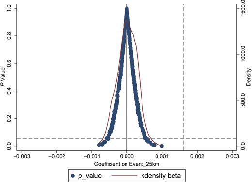
Placebo test. Note(s): This figure shows a distribution of the estimated coefficients for Pseudo_Event_25km, derived from 500 iterations of placebo tests where we replace Event_25km with randomly generated pseudo-event dates (Pseudo_Event) and randomly selected treatment and control firms (Pseudo_Treat) in the baseline regression. Source(s): Figure created by authors
Placebo test. Note(s): This figure shows a distribution of the estimated coefficients for Pseudo_Event_25km, derived from 500 iterations of placebo tests where we replace Event_25km with randomly generated pseudo-event dates (Pseudo_Event) and randomly selected treatment and control firms (Pseudo_Treat) in the baseline regression. Source(s): Figure created by authors
3.4 Channel analyses
In developing our argument, we propose two mechanisms by which the outbreak of extreme environmental events leads to an increase in the cost of debt: (1) stricter local government environmental enforcement and monitoring and (2) an increase in the risk of firm operation. In this section, we test each channel and report the results in Table 6.
Channel analyses
| Panel A: local environmental enforcement and monitoring | ||
|---|---|---|
| Dependent variable | (1) | (2) |
| EnvirPer | EnvirAct | |
| Event_25km | 0.029** | 0.010*** |
| (2.131) | (3.907) | |
| Size | 0.002 | 0.001 |
| (0.297) | (0.633) | |
| Lev | −0.013 | −0.002 |
| (−0.687) | (−0.385) | |
| PPE | 0.120*** | 0.007 |
| (3.558) | (0.965) | |
| CFO | −0.030 | −0.004 |
| (−0.841) | (−0.439) | |
| Age | −0.057*** | −0.005* |
| (−3.529) | (−1.926) | |
| SOE | −0.041** | −0.001 |
| (−2.554) | (−0.281) | |
| ROA | −0.003 | −0.004 |
| (−0.073) | (−0.403) | |
| Board | 0.048* | 0.018*** |
| (1.815) | (3.103) | |
| SalesGrowth | −0.005 | −0.001 |
| (−1.393) | (−1.078) | |
| Block | −0.036 | −0.013 |
| (−0.792) | (−1.488) | |
| Cons | 1.297*** | 0.119*** |
| (9.373) | (4.288) | |
| Firm FE | Yes | Yes |
| Year FE | Yes | Yes |
| Observations | 23,162 | 23,162 |
| Adj. R2 | 0.137 | 0.140 |
| Panel B: operation risk | ||
|---|---|---|
| Dependent variable | (1) | (2) |
| Risk_roa | Risk_cfo | |
| Event_25km | −0.001 | −0.001 |
| (−0.860) | (−0.533) | |
| Size | −0.006*** | −0.008*** |
| (−6.169) | (−8.784) | |
| Lev | 0.038*** | 0.020*** |
| (10.366) | (5.800) | |
| PPE | −0.011** | −0.034*** |
| (−2.476) | (−9.949) | |
| CFO | 0.018*** | 0.013** |
| (3.909) | (2.423) | |
| Age | 0.005*** | 0.004*** |
| (5.775) | (3.834) | |
| SOE | −0.005* | −0.002 |
| (−1.877) | (−1.214) | |
| ROA | −0.204*** | 0.008 |
| (−28.635) | (1.445) | |
| Board | 0.005 | −0.001 |
| (1.377) | (−0.487) | |
| SalesGrowth | −0.001** | 0.003*** |
| (−2.330) | (4.696) | |
| Block | −0.041*** | 0.011** |
| (−6.755) | (2.360) | |
| Cons | 0.157*** | 0.206*** |
| (7.927) | (11.379) | |
| Firm FE | Yes | Yes |
| Year FE | Yes | Yes |
| Observations | 34,299 | 33,113 |
| Adj. R2 | 0.257 | 0.042 |
Note(s): This table presents the results of the channel tests. In Panel A, we examine the regulatory risk channel. The dependent variables are EnvirPer and EnvirAct. EnvirPer is defined as the proportion of words in the government work report that reflect the extent how seriously the government takes the environment. EnvirAct is defined as the proportion of words in the government work report that can reflect the actions taken by the local government to protect the environment. In Panel B, we examine the operating risk channel. The dependent variables are Risk_roa and Risk_cfo. Risk_roa is the standard deviation of industry-adjusted ROA over the next three years. Risk_cfo is the standard deviation of cash flow over the next three years. Variable definitions are provided in Supplementary material. The regressions are performed using OLS. The t-statistics in parentheses are adjusted for heteroscedasticity and clustered by firm. ***, ** and * indicate significance at the 1%, 5% and 10% levels, respectively
Source(s): Table created by authors
3.4.1 Local environmental enforcement and monitoring
In our first channel test, we investigated whether local environmental enforcement and monitoring increased in response to the outbreak of extreme environmental events. We follow prior studies (e.g. Barnard & Simon, 1947; Ocasio, 1997) and use two city-level indicators to measure the level of local environmental enforcement and monitoring. The first variable is EnvirPer, defined as the percentage of words in the government work report that reflect the level of importance the government places on environmental protection. Similar to Chen, Kahn, Liu, and Wang (2018), the related keyword includes a total of 101 words about environmental protection, environmental pollution, energy consumption, coordinated development and environmental co-governance. The second variable is EnvirAct, which is defined as the percentage of words in the government work report that can reflect the actions taken by the local government to protect the environment. Similarly, the corresponding keywords include environmental protection inspection, pollution prevention and control, joint prevention, joint control, joint governance, emission reduction, environmental protection coordination, collaborative pollution control, departmental cooperation, public participation, clean land, sewage treatment, conservation, etc. The above keywords comprehensively measure the strength of local government environmental governance. In addition, the local government generally issues its work report at the beginning of the year and the economic outcome during the year is unlikely to affect the government work report that has been determined in advance, which helps to alleviate the endogenous problems (Chen et al., 2018). A higher value of EnvirPer and EnvirAct indicates stricter local government environmental enforcement and monitoring. We re-estimate the regression in Equation (1) by replacing Debtcost with EnvirPer or EnvirAct and report the results in Panel A of Table 6. The dependent variable is EnvirPer in Column (1) and the coefficient on Event_25k is positive and significant at the 5% level. Column (2) also shows that the coefficient on Event_25k is 0.010 and significant at the 1% level when the dependent variable is EnvirAct. In sum, the findings show that the outbreak of extreme environmental events indeed increases local government environmental enforcement and monitoring.
3.4.2 Operating risk
The second channel we propose for the impact of the outbreak of extreme environmental events on the cost of debt is the potential increase in firm operation risk. Following John, Litov, and Yeung (2008), we use two measures to capture the operational risk of the firm: Risk_roa and Risk_cfo. Risk_roa is the standard deviation of industry-adjusted ROA over the next three years, where ROA is equal to EBIT divided by total assets at the end of the year. Risk_cfo is the standard deviation of cash flow over the next three years, where cash flow is equal to operating cash flow divided by total assets at the end of the year. We re-estimate the regression in Equation (1) by replacing Debtcost with Risk_roa or Risk_cfo. The results are reported in Panel B of Table 6. Columns (1) and (2) show that the coefficients of Event_25k are insignificant when the dependent variables are Risk_roa and Risk_cfo. These results indicate that the outbreak of local extreme environmental events does not increase the operating risk of treatment firms.
In sum, our channel tests indicate that the outbreak of extreme environmental events increases the cost of debt through increased environmental enforcement and local government monitoring.
3.5 Cross-sectional analyses
3.5.1 Extent and severity of the extreme environmental events
Thus far, we have documented that the outbreak of extreme environmental events increases the cost of debt of treatment firms located near the place where extreme environmental events happened. It is unclear whether the extent and severity of the extreme environmental events exaggerate the increase in the cost of debt. Bordalo, Gennaioli, and Shleifer (2013) indicated that rare events are often overweighted when the outcomes are significant and underweighted when the outcomes are moderate. According to the severity of the consequences caused by the emergent event (e.g. casualties, economic losses, ecological damage, water pollution, radiation pollution, cross-border consequences), the government classifies extreme environmental events into four categories: “particularly significant”, “significant”, “major” and “general”. We define two dummy variables to capture the seriousness of the extreme environmental events. Rank is equal to one if the extreme environmental event is classified as the top one level (“particularly significant”), and zero otherwise. Rank1 is equal to one if the extreme environmental event is classified as the top three levels (“particularly significant”, “significant” and “major”), and zero otherwise.
The result is reported in Panel A of Table 7. In column (1), the coefficient for the interaction term Event_25km × Rank is 0.003 and significant at the 5% level. Column (2) shows that the coefficient on Event_25km × Rank1 is 0.005 and significant at the 1% level [3]. The results suggest that the increase in the cost of debt is more pronounced for firms that are exposed to more severe local extreme environmental events.
Cross-sectional tests
| Dependent variable | (1) | (2) |
|---|---|---|
| Debtcost | Debtcost | |
| Panel A: extent and severity of the extreme environmental events | ||
| Event_25km | −0.000 | 0.001 |
| (−0.016) | (0.828) | |
| Event_25km × Rank | 0.003** | |
| (2.507) | ||
| Event_25km × Rank1 | 0.005*** | |
| (2.668) | ||
| Size | 0.004*** | 0.004*** |
| (9.902) | (9.904) | |
| Lev | 0.026*** | 0.026*** |
| (10.606) | (10.566) | |
| PPE | 0.038*** | 0.038*** |
| (15.994) | (15.935) | |
| CFO | −0.025*** | −0.025*** |
| (−11.813) | (−11.819) | |
| Age | 0.011*** | 0.011*** |
| (15.497) | (15.399) | |
| SOE | −0.003*** | −0.003*** |
| (−2.627) | (−2.644) | |
| ROA | −0.015*** | −0.015*** |
| (−5.662) | (−5.650) | |
| Board | −0.001 | −0.001 |
| (−0.969) | (−0.846) | |
| SalesGrowth | 0.000** | 0.000** |
| (2.015) | (2.037) | |
| Block | −0.005* | −0.005* |
| (−1.702) | (−1.731) | |
| Cons | −0.102*** | −0.102*** |
| (−10.743) | (−10.770) | |
| Firm FE | Yes | Yes |
| Year FE | Yes | Yes |
| Observations | 34,833 | 34,833 |
| Adj. R2 | 0.188 | 0.188 |
| Dependent variable | (1) | (2) | (3) | (4) |
|---|---|---|---|---|
| Debtcost | Debtcost | Debtcost | Debtcost | |
| Panel B: environmental performance | ||||
| Event_25km | 0.002** | 0.002** | 0.002** | 0.002** |
| (2.473) | (2.281) | (2.093) | (2.308) | |
| EPtConcept | −0.000 | |||
| (−0.501) | ||||
| Event_25km × EPtConcept | −0.002** | |||
| (−2.389) | ||||
| EPHonorReward | 0.000 | |||
| (0.656) | ||||
| Event_25km × EPReward | −0.003*** | |||
| (−3.924) | ||||
| EPSpecialAct | −0.000 | |||
| (−0.103) | ||||
| Event_25km × EPAct | −0.002** | |||
| (−2.083) | ||||
| EmergMech | −0.001** | |||
| (−2.086) | ||||
| Event_25km × EmergMech | −0.002** | |||
| (−2.482) | ||||
| Size | 0.004*** | 0.004*** | 0.004*** | 0.004*** |
| (7.214) | (7.167) | (7.180) | (7.118) | |
| Lev | 0.036*** | 0.036*** | 0.036*** | 0.036*** |
| (13.338) | (13.343) | (13.343) | (13.350) | |
| PPE | 0.044*** | 0.044*** | 0.044*** | 0.044*** |
| (15.716) | (15.734) | (15.696) | (15.800) | |
| CFO | −0.026*** | −0.026*** | −0.026*** | −0.026*** |
| (−10.548) | (−10.521) | (−10.563) | (−10.531) | |
| Age | 0.013*** | 0.013*** | 0.013*** | 0.013*** |
| (15.885) | (15.904) | (15.910) | (15.876) | |
| SOE | −0.002 | −0.002 | −0.002 | −0.002 |
| (−1.192) | (−1.209) | (−1.202) | (−1.269) | |
| ROA | −0.008** | −0.008** | −0.008** | −0.008** |
| (−2.529) | (−2.530) | (−2.552) | (−2.453) | |
| Board | −0.001 | −0.001 | −0.001 | −0.001 |
| (−0.443) | (−0.438) | (−0.471) | (−0.491) | |
| SalesGrowth | 0.001** | 0.001** | 0.001** | 0.001*** |
| (2.514) | (2.544) | (2.525) | (2.583) | |
| Block | −0.000 | −0.001 | −0.001 | −0.001 |
| (−0.146) | (−0.165) | (−0.164) | (−0.229) | |
| Cons | −0.113*** | −0.112*** | −0.113*** | −0.112*** |
| (−9.744) | (−9.702) | (−9.692) | (−9.618) | |
| Firm FE | Yes | Yes | Yes | Yes |
| Year FE | Yes | Yes | Yes | Yes |
| Observations | 28,180 | 28,180 | 28,180 | 28,180 |
| Adj. R2 | 0.192 | 0.192 | 0.191 | 0.192 |
| Dependent variable | (1) | (2) |
|---|---|---|
| Debtcost | Debtcost | |
| Panel C: ESG rating score | ||
| Event_25km | 0.003*** | 0.002*** |
| (3.155) | (2.630) | |
| ESG_Env | 0.001*** | |
| (2.959) | ||
| Event_25km × ESG_Env | −0.003*** | |
| (−3.145) | ||
| ESG | −0.000 | |
| (−0.454) | ||
| Event_25km × ESG | −0.002** | |
| (−2.060) | ||
| Size | 0.003*** | 0.003*** |
| (5.340) | (5.515) | |
| Lev | 0.045*** | 0.045*** |
| (17.390) | (17.347) | |
| PPE | 0.044*** | 0.044*** |
| (14.733) | (14.739) | |
| CFO | −0.026*** | −0.026*** |
| (−10.190) | (−10.252) | |
| Age | 0.013*** | 0.013*** |
| (15.487) | (15.503) | |
| SOE | −0.003* | −0.003* |
| (−1.937) | (−1.874) | |
| ROA | −0.006** | −0.006** |
| (−2.124) | (−2.076) | |
| Board | −0.001 | −0.001 |
| (−0.491) | (−0.582) | |
| SalesGrowth | 0.001** | 0.001** |
| (2.097) | (2.035) | |
| Block | −0.001 | −0.001 |
| (−0.400) | (−0.381) | |
| Cons | −0.101*** | −0.102*** |
| (−8.054) | (−8.143) | |
| Firm FE | Yes | Yes |
| Year FE | Yes | Yes |
| Observations | 28,568 | 28,568 |
| Adj. R2 | 0.198 | 0.198 |
| Panel D: relationship with the government | ||
| Event_25km | 0.003*** | 0.003*** |
| (3.083) | (2.889) | |
| SOE | −0.002* | −0.003** |
| (−1.756) | (−2.563) | |
| Event_25km × SOE | −0.004*** | |
| (−2.933) | ||
| Size_Ind | −0.001** | |
| (−2.219) | ||
| Event_25km × Size_Ind | −0.002** | |
| (−2.334) | ||
| Size | 0.004*** | 0.005*** |
| (9.870) | (10.442) | |
| Lev | 0.026*** | 0.026*** |
| (10.681) | (10.680) | |
| PPE | 0.038*** | 0.038*** |
| (15.963) | (15.981) | |
| CFO | −0.025*** | −0.025*** |
| (−11.862) | (−11.889) | |
| Age | 0.011*** | 0.011*** |
| (15.236) | (15.606) | |
| ROA | −0.015*** | −0.015*** |
| (−5.514) | (−5.518) | |
| Board | −0.001 | −0.001 |
| (−0.935) | (−0.950) | |
| SalesGrowth | 0.000** | 0.000** |
| (2.011) | (2.008) | |
| Block | −0.004* | −0.005* |
| (−1.663) | (−1.826) | |
| Cons | −0.102*** | −0.114*** |
| (−10.780) | (−11.214) | |
| Firm FE | Yes | Yes |
| Year FE | Yes | Yes |
| Observations | 34,833 | 34,833 |
| Adj. R2 | 0.188 | 0.188 |
Note(s): This table presents the results of cross-sectional variations. We examine the moderating effect of the extent of extreme environmental events, environmental performance and the relationship with the government. Variable definitions are provided in Supplementary material. The regressions are performed using OLS. The t-statistics in parentheses are adjusted for heteroscedasticity and clustered by firm. *, ** and *** denote statistical significance at the 10%, 5% and 1% levels, respectively
Source(s): Table created by authors
3.5.2 Environmental performance
We explore whether the relationship between extreme environmental events and the cost of debt varies with firms’ environmental performance. If firms disclose more environmental information or perform better in terms of environmental performance, the information asymmetry between firms and the government will be reduced. It further reduces the possibility that firms are subject to ongoing and strict government monitoring, especially when extreme environmental events occur near the headquarters of the firm. Prior studies (e.g. Cooper & Uzun, 2015; Eichholtz et al., 2019; Chen et al., 2021) also suggest that better corporate environmental performance is significantly associated with lower debt costs. Thus, we expect that the impact of extreme environmental events on the cost of debt will be attenuated by firms with better environmental performance.
To test this prediction, we used four variables to capture the transparency of environmental information and environmental performance based on the information in the annual report. First, EPtConcept is a dummy variable that equals one if the firm discloses environmental protection philosophy, environmental policy, environmental management organizational structure, circular economy development model, green development, etc. and zero otherwise. Second, EPReward is a dummy variable that equals one if the firm discloses the honor or award it has received for environmental protection and zero otherwise. Third, EPAct is a dummy variable that equals one if the firm discloses its participation in special environmental protection activities, environmental protection and other social welfare activities, and zero otherwise. Fourth, EmergMech is a dummy variable that equals one if the firm discloses establishing an emergency response mechanism for major environment-related events, the measures taken in response to the emergency, the treatment method of pollutants, etc. and zero otherwise. We interact these four variables separately with Event_25k, and include the interaction term in the regression specification in Equation (1). Panel B of Table 7 reports the results.
In columns (1)–(4), the coefficients of the interaction terms (Event_25km×EPtConcept, Event_25km×EPReward, Event_25km×EPAct and Event_25km×EmergMech) are all significantly negative. The results indicate that the relationship between the outbreak of extreme environmental events and debt cost is more significant among firms with lower transparency of environmental information or worse environmental performance.
Next, we also use firms’ ESG rating scores to capture corporate environmental performance. We use the ESG rating score developed by Shanghai Huazheng Index Information Service Co., Ltd. ESG is a dummy variable that equals one if the firm’s ESG rating score is higher than the median of the sample year and zero otherwise. ESG_Env is a dummy variable that equals one if the ESG environment dimension rating score is higher than the median of the sample year and zero otherwise. We separately interact ESG and ESG_Env with Event_25k, and include the interaction term in the regression specification in Equation (1). The results are reported in Panel C of Table 7. The coefficients of the interaction terms Event_25km×ESG and Event_25km×ESG_Env are all significantly negative. These results show that the adverse effect of the outbreak of extreme environmental events on the cost of debt is weakened for firms with higher environmental dimension ESG rating scores.
3.5.3 Relation with the government
We evaluate whether the relationship between extreme environmental events and the cost of debt hinges on firms’ relations with the government. We argue that extreme local environmental events could incur stricter environmental monitoring, which increases the compliance costs faced by the local firms. However, suppose the treatment firms have a good relationship or connection with the local government. In that case, they may better understand the new environmental policy and avoid future environmental violations and punishment. Thus, we expect that the adverse effect of extreme environmental events on the cost of debt will be weakened for firms with a relationship with the government. Following prior papers (e.g. Wu, Wang, Luo, & Gillis, 2012; Salamon & Siegfried, 1977; Richardson & Lanis, 2007), SOEs and bigger firms have stronger lobbying power and are more involved in policy participation. For example, firms that have better relations with the government have lower effective tax rates. Thus, we use SOEs and firm status (Size_Ind) to capture the relationship between the firm and the government. Size_Ind is a dummy variable equal to 1 if the firm’s total assets are larger than the median value by industry and year (high firm status), and zero otherwise (low firm status). We separately interact SOE and Size_Ind with Event_25k and include the interaction term in the regression specification in Equation (1). The results are reported in Panel D of Table 7. We find that the coefficients of the interaction terms Event_25km×SOE and Event_25km×Status are all significantly negative. These results demonstrate that the increase in debt cost is weakened in SOEs and bigger firms that are exposed to local outbreaks of extreme environmental events.
4. Economic consequences
In this section, we conduct two additional analyses to further explore the economic consequences caused by local extreme environmental events. The first test focuses on corporate cash holding, and the second focuses on investment expenditure.
4.1 Cash holding
Our evidence suggests an adverse impact of local extreme environmental events on the cost of debt. To deepen our analysis, we explore whether treatment firms increase their cash holding in response to the increase in the cost of debt caused by extreme environmental events. Cash holding (Cashhold) is the monetary capital and net value of short-term investment divided by net assets. We regress cash holding measures on the interaction terms Event_25km ×Debtcost, Event_25km, Debtcost and a series of control variables. The results reported in Panel A of Table 8 show that the coefficient on the interaction term Event_25km × Debtcost is 0.747 and significant at the 1% level. The result suggests that treatment firms increase their cash holding in response to the increased cost of debt caused by extreme environmental events.
Economic consequences
| Panel A: cash holding | |
|---|---|
| Dependent variable | (1) |
| Cashhold | |
| Event_25km ×Debtcost | 0.747*** |
| (2.747) | |
| Event_25km | −0.007 |
| (−0.866) | |
| Debtcost | −3.578*** |
| (−20.407) | |
| Size | −0.037*** |
| (−6.367) | |
| Lev | 0.038* |
| (1.686) | |
| PPE | −0.138*** |
| (−6.713) | |
| CFO | 0.223*** |
| (8.471) | |
| Age | −0.055*** |
| (−9.486) | |
| SOE | 0.007 |
| (0.433) | |
| ROA | 0.005 |
| (0.137) | |
| Board | 0.029* |
| (1.891) | |
| Sales Growth | 0.005 |
| (1.593) | |
| Block | −0.013 |
| (−0.432) | |
| Cons | 1.037*** |
| (8.243) | |
| Firm FE | Yes |
| Year FE | Yes |
| Observations | 34,830 |
| Adj. R2 | 0.195 |
| Panel B: investment expenditure | |||
|---|---|---|---|
| Dependent variable | (1) | (2) | (3) |
| InvestNet | RD | Patent | |
| Event_25km ×Debtcost | −0.054** | −0.017** | −1.848*** |
| (−1.973) | (−1.995) | (−2.904) | |
| Event_25km | 0.001 | 0.001 | 0.073** |
| (0.487) | (1.558) | (2.080) | |
| Debtcost | −0.016 | 0.007 | −0.688** |
| (−0.965) | (1.416) | (−2.014) | |
| Size | 0.001* | −0.000 | 0.317*** |
| (1.815) | (−0.238) | (14.774) | |
| Lev | −0.015*** | −0.001 | 0.145** |
| (−5.798) | (−1.260) | (2.498) | |
| PPE | −0.055*** | 0.002* | 0.150 |
| (−10.818) | (1.864) | (1.548) | |
| CFO | 0.037*** | 0.004*** | −0.097 |
| (8.671) | (3.935) | (−1.127) | |
| Age | −0.013*** | −0.001** | 0.052** |
| (−11.860) | (−2.073) | (1.977) | |
| SOE | −0.002 | 0.000 | 0.091* |
| (−0.823) | (0.501) | (1.827) | |
| ROA | 0.046*** | 0.001 | 0.576*** |
| (10.709) | (0.443) | (7.025) | |
| Board | 0.005 | 0.001 | 0.117* |
| (1.449) | (0.935) | (1.676) | |
| SalesGrowth | 0.001*** | 0.000*** | −0.013 |
| (2.751) | (2.897) | (−1.364) | |
| Block | 0.010* | −0.006*** | −0.500*** |
| (1.726) | (−3.202) | (−3.457) | |
| Cons | 0.051*** | 0.008 | −6.334*** |
| (3.054) | (1.546) | (−13.693) | |
| Firm FE | Yes | Yes | Yes |
| Year FE | Yes | Yes | Yes |
| Observations | 33,311 | 33,329 | 33,329 |
| Adj. R2 | 0.125 | 0.162 | 0.295 |
Note(s): This table examines the economic consequences caused by local extreme environmental events. In Panel A, we focus on corporate cash holding. Cashhold is measured as monetary capital and the net value of short-term investment divided by net assets. In Panel B, we focus on the input and output of investment expenditure. InvestNet is cash paid to acquire fixed assets, intangible assets and other long-term assets, minus net cash received from the disposal of fixed assets, intangible assets and other long-term assets, divided by total assets. R&D expenses RD are R&D expenses divided by total assets. Patent is the natural logarithm of the number of invention patent applications plus 1. Variable definitions are provided in Supplementary material. The regressions are performed using OLS. The t-statistics in parentheses are adjusted for heteroscedasticity and clustered by firm. ***, ** and * indicate significance at the 1%, 5% and 10% levels, respectively
Source(s): Table created by authors
4.2 Investment expenditure
Next, we examine whether treatment firms deduct investment expenditures considering the increased cost of debt due to local extreme environmental events. Following prior papers (e.g. Richardson, 2006; Gao & Chou, 2015; Hall & Harhoff, 2012; Tong, He, He, & Lu, 2014), we use three measures to capture the input and output of investment expenditure. Net investment expenditure (InvestNet) is cash paid to acquire fixed assets, intangible assets and other long-term assets minus net cash received from the disposal of fixed assets, intangible assets and other long-term assets, divided by total assets. R&D expenses (RD) are R&D expenses divided by total assets. Invention patent (Patent) is the natural logarithm of the number of invention patent applications plus 1. We regress investment expenditure measures on the interaction terms Event_25km × Debtcost, Event_25km, Debtcost and a series of control variables. The results are reported in Panel B of Table 8. In columns (1)-(3), the coefficients of the interaction term Event_25km × Debtcost are all negative and significant, consistent with our expectation that treatment firms reduce the input and output of investment expenditure after the outbreak of extreme environmental events. In sum, the above results imply that extreme environmental events impede the long-term development of the firms.
5. Conclusion
In this paper, we examine whether firms’ environmental risk, captured by local extreme environmental events, increases the cost of debt. We propose that the outbreak of local extreme environmental events may trigger stricter local government environmental enforcement and supervision, increasing the compliance costs of firms exposed to such extreme environmental events. However, it is also possible that extreme environmental events increase the awareness of environmental risk management for local firms, reducing the uncertainty of corporate operations. Therefore, whether local extreme environmental events increase the cost of debt is an empirical question.
Using difference-in-differences research design, we find that treated firms exposed to extreme environmental events near their headquarters have a higher cost of debt. Our results hold for a parallel trend test and several robustness checks. Additionally, we find that the outbreak of extreme environmental events increases the percentage of words related to the importance of the environment and environmental protection actions in the government work report, suggesting an increase in local government environmental enforcement and supervision. This evidence supports our argument that the outbreak of extreme environmental events increases the cost of debt through strengthened local government environmental enforcement and supervision. Furthermore, we find that the positive relationship between the outbreak of extreme environmental events and the cost of debt is weaker for firms exposed to less severe local extreme environmental events, firms with better environmental performance, and firms with a relationship with the government. Last, we show that treatment firms increase their cash holding and investment expenditure in response to the increased cost of debt caused by extreme environmental events, suggesting that extreme environmental events have an adverse impact on the long-term development of the firms.
By documenting the adverse impact of extreme environmental events on the cost of debt, our study contributes to the literature on the role of environmental risk and performance and the literature on the determinants of the cost of debt. Given that debt financing is significantly important for firms in emerging countries, our findings suggest that firms should disclose more information related to environmental actions or perform better in terms of the environment to attenuate the adverse impact caused by exogenous environmental risk shocks. Further research may examine treatment firms’ response to extreme local environmental events. Further research may also consider whether the increase in the cost of debt caused by extreme exogenous environmental events is reasonable or beneficial for the overall economic development in the local area, given that the operational risk of treatment firms does not change.
We greatly appreciate helpful comments and suggestions from Yuan Huang, Chuang Lu, Cheng Zeng and seminar participants at Central University of Finance and Economics. Xiao Li acknowledges financial support from the National Natural Science Foundation of China (#72472170). Xin Yang acknowledges financial support from the National Natural Science Foundation of China (#72402245), the Chenguang Program of Shanghai Education Development Foundation and Shanghai Municipal Education Commission, the Fundamental Research Funds for the Central Universities and the Shanghai Pujiang Programme. All errors are ours.
Notes
This is based on statistics on debt financing obtained from the World Development Indicators of the World Bank. Source: https://databank.worldbank.org/source/world-development-indicators
The local government began to disclose environmental emergencies data in 2004.
The regression coefficients for Rank and Rank1 are not shown in the table and are automatically removed due to collinearity.
References
The supplementary material for this article can be found online.
