

The simulation of eddy currents in laminated iron cores by the finite element method (FEM) is of great interest in the design of electrical devices. Modeling each laminate by finite elements leads to extremely large nonlinear systems of equations impossible to solve with present computer resources reasonably. The purpose of this study is to show that the multiscale finite element method (MSFEM) overcomes this difficulty.
A new MSFEM approach for eddy currents of laminated nonlinear iron cores in three dimensions based on the magnetic vector potential is presented. How to construct the MSFEM approach in principal is shown. The MSFEM with the Biot–Savart field in the frequency domain, a higher-order approach, the time stepping method and with the harmonic balance method are introduced and studied.
Various simulations demonstrate the feasibility, efficiency and versatility of the new MSFEM.
The novel MSFEM solves true three-dimensional eddy current problems in laminated iron cores taking into account of the edge effect.
1. Introduction
A laminated core represents a periodic micro-structure which is well suited for the multiscale finite element method (MSFEM). The aim of MSFEMs is to reduce the computational costs of eddy currents in very large laminated iron cores drastically without losing accuracy (Dular, 2008; Hollaus and Schöberl, 2018).
It can be stated that MSFEMs for eddy currents in laminated iron in two dimensions (2D) are well established. Problems in 2D have been solved very satisfactorily using a magnetic vector potential (MVP) A, a current vector potential T or a the mixed formulation with A and the current density J, see (Hollaus and Schöberl, 2018).
However, MSFEMs for three-dimensional (3D) problems are still far away from being a satisfactory solution. Analyzing the numerical examples in the literature it is very striking to see that there have been no real 3D MSFEM simulations presented up to now. Most of the examples are rotationally symmetric, for instance a toroidal transformer (Gyselinck et al., 2006), or the magnetic flux is parallel to the laminates (Dular, 2008). Both kinds of problems exhibit no magnetic stray fields.
MSFEMs for 3D problems can be divided into methods solving real 3D problems and those considering 2D/1D-problems. The 2D/1D-MSFEMs are based on the assumption that the end effects of electrical machines, i.e. magnetic stray fields can be neglected; thus, each laminate is exposed to the same electromagnetic field distribution and therefore a simulation of a single laminate suffices, (Bottauscio and Chiampi, 2002; Rasilo et al., 2011). A 2D problem is solved essentially reducing the computational costs compared to brute force 3D finite element method (FEM) models (Handgruber et al., 2013; Schöbinger et al., 2018).
The present paper deals with problems where this assumption is not applicable and 3D problems have to be solved. The aim of this work is to present a novel MSFEM for laminated iron stacks in 3D and its universal applicability and efficiency compared to the standard finite element method (SFEM). This MSFEM is based on A. After recalling the analytic solution of eddy currents in an infinite slab the construction of the basic MSFEM approach with A will be discussed in detail. Different aspects like averaging of coefficients and the edge effect are addressed. The method is capable to consider air gaps and the edge effect too.
Simulation results obtained by all specific MSFEMs will be shown and compared to reference solutions computed by the standard finite element method (SFEM) demonstrating the versatility of the new MSFEM for problems in 3D. The savings in computational costs using the new MSFEM instead of SFEM are presented at the end.
2. The multiscale finite element method – MSFEM
A laminated iron core exhibits two very different scales. The large scale is determined by the overall dimensions of a laminated core, e.g. the length L and the height H of a transformer core as shown in Figure 1 on the left, and the small (micro-) scale determined by the tiny dimensions of the thickness of the laminates d and the width of an air gap d0 in between, see Figure 1 on the right. The ratio of these scales is about 106, and thus very large. Modeling each laminate and air gap of large electrical devices would yield a very large finite element model and consequently an extremely large equation system impossible to solve with reasonable computational effort. However, a laminated iron core represents a quasi-periodic structure, this means not strictly periodic because of the finite overall dimensions, which can be exploited by the MSFEM advantageously. One period p is composed of d and d0.
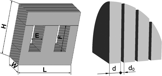
Large scale: transformer core with overall dimensions (left), Fine scale: thickness of the laminate d and width of the air gap d0 (right)
Large scale: transformer core with overall dimensions (left), Fine scale: thickness of the laminate d and width of the air gap d0 (right)
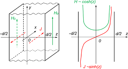
To substantiate the MSFEM approach, the exact solution of eddy currents in an infinite slab is highly relevant and for convenience the main results are summarized in the following (Stoll, 1974). A Cartesian coordinate system is used.
A single component MVP A = Aex is assumed to be selected at the surfaces z = ±d/2 of the slab prescribing a magnetic flux per unit length, such that the magnetic field H points into the y-direction inducing eddy currents pointing into the x-direction, i.e. H = Hey and J = Jex, respectively, see Figure 2. On the other hand J = −jωσA holds.
Provided the linear problem is given in the frequency domain, the quasi-static magnetic field with the phasor convention ejωt reads as:
with the solution:
where:
Holds. The solution (2) is described by a hyperbolic sine which is an odd function. Therefore, odd Gauss–Lobatto polynomials
are used for micro-shape functions ϕi(s) to construct MSFEM approaches with A. The transformation s = 2z/d holds with s∈[−1,1] and z∈[−d/2,d/2]. The micro-shape functions ϕi are extended by zero in [−(d0+d)/2,−d/2] and [d/2,(d0+d)/2] including the air gap, except ϕ1 which is extended linearly and becomes zero in {−(d0+d)/2,(d0+d)/2}. Figure 3 shows how the micro-shape functions ϕi fit into the periodic structure with d and d0.
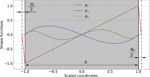
Gauss–Lobatto polynomials are the micro-shape functions, scaled s ∈ (Dular, 2008), the laminate is grey
Gauss–Lobatto polynomials are the micro-shape functions, scaled s ∈ (Dular, 2008), the laminate is grey
Thus, the polynomials facilitate the required continuity of the unknown solution, ϕi (–1) = 0 and ϕi (1) = 0 with i = 3, 5.
2.1 Construction of a multiscale finite element method approach with A
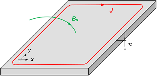
To construct a MSFEM approach with A, the eddy currents of a reference solution, detailed in Figure 4, are studied.
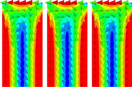
Eddy currents due to the main magnetic flux in laminates with the edge effect, detail
Eddy currents due to the main magnetic flux in laminates with the edge effect, detail
Based on the eddy current distribution, the approach:
is found. The first term A0 in (4) describes the large-scale behavior of the solution, whereas the others that of the fine scale. The large-scale behavior takes account of the large eddy current loops induced by the magnetic stray flux perpendicular to the lamination (Figure 5). At the fine scale, the main magnetic flux parallel to the lamination induces eddy currents confined to flow in very narrow loops shown in Figure 6. These currents are assumed to be split into two parts. The laminar part which is parallel to the laminates and represented by the second term in equation (4), the third term includes the edge effect, i.e. the part where the currents turn around to form closed loops (Figure 6).
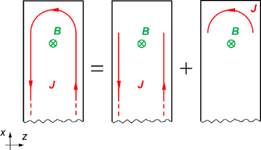
Main magnetic flux (green) and a narrow eddy current loop (red) in a small part at the end of a laminate, fictitious decomposition of the current density
Main magnetic flux (green) and a narrow eddy current loop (red) in a small part at the end of a laminate, fictitious decomposition of the current density
The boundary value problem to be solved is the ECP:
where Ωc represents the conducting domain (iron) and Ω0 the non-conducting domain (air). The weak form is:
Find , such that
for all vh∈V0, where Vh⊂H(curl,Ω).
For a unique solution the regularization with 0<σ0⪡σ is applied (Ledger and Zaglmayr, 2010). The solution of equation (6) with the SFEM serves as reference solution for the MSFEM. To end up with a weak form for the MSFEM, equation (4) becomes the trial function and
the test function with the same structure. Tilde marks the multiscale approach. The laminated domain Ωm consists of the iron laminates and the air gaps. A1, w1 and ϕ1 are restricted to Ωm, whereas A0 is valid in the entire domain Ω=Ωm∪Ω0. Dirichlet and thus essential boundary conditions are prescribed by means of A0 exclusively, and only natural boundary conditions are provided for A1 and w1. This is especially true for planes of symmetry. To obtain the weak form for the MSFEM, simply speaking, Ah and vh in the weak form of the SFEM [equation (6)] are replaced by A˜h and v˜h, respectively, resulting in:Find such that:
for all (v0h, v1h, q1h)∈V0, where Uh⊂H(curl,Ω), Vh⊂H(curl,Ωm) and Wh⊂H1(Ωm) have been selected. The micro-shape function ϕ1 is a periodic, piecewise linear and continuous function, i.e. ϕ1∈Hper(Ωm).
2.2 Averaging of the highly oscillating coefficients
The arising highly oscillating coefficients in equation (8) make the finite element assembling very expensive. To overcome this problem these coefficients are averaged. Here, the stiffness term is treated representing the mass term too. Writing the stiffness term in detail yields:
and carrying out the multiplications leads to:
Analogue operations are carried out also for the mass term of equation (8).
Coefficients , etc. and σ, σϕ1,z, σϕ1, etc. are averaged over the period p = d + d0:
where λ means either or σ in iron or air. The bar marks averaging.
Highly oscillating coefficients are replaced by averaged ones, whereby the bilinear form and the linear form in
modifying the unknown quantities indicated by the bar. The error due to averaging is assumed to be negligibly small (Hollaus and Schöberl, 2018).
The averaged coefficients are constant and therefore a rather coarse FE-mesh suffices to get an accurate approximation of the solution. In fact, equations (8) and (10) are solved.
2.3 Biot–Savart field and multiscale finite element method
Fields due to currents in coils can be considered by the Biot–Savart field. Rearranging of the linear form yields:
where hS is the Biot-Savart-field
of the unit current. By averaging only v0h remains as test function for the linear form.
3. Numerical example
The single phase transformer shown in Figure 7 is used to study various simulations of different MSFEMs. The core consists of 183 laminates yielding a fill-factor of kf = 0.9734. An electric conductivity of σ = 2.0 · 106 S/m and a relative permeability of μr = 1,000 in the linear case have been selected. The cross-section of a cylindrical coil is shown in Figure 8. It consists of two layers (dark rings), 60 turns per layer. The length of the coil equals 192 mm. The arrangement of the core with the coils exhibit three planes of symmetry.
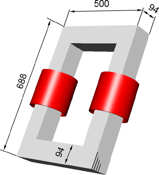
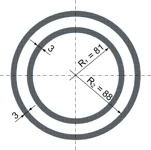
A handmade mesh was created by means of hexahedral FEs to simplify the modeling of each laminate for the reference solution. The Biot–Savart field was used to avoid the modeling of the cylindrical coils. Due to the symmetry one eighth of the problem has been considered in the simulations.
4. Different simulations
4.1 Frequency domain and higher-order multiscale finite element method
We start with the linear case in the frequency domain and show how to cope with small penetration depths making use of higher-order MSFEM (HMSFEM). To this end, the basic approach [equation (4)] is extended by adding higher order micro-scale terms (Hollaus and Schöberl, 2015), leading to:
Figure 9 shows the eddy current losses computed by SFEM and MSFEM. The relative error of MSFEM presented in Figure 10 is obtained by comparing to SFEM results which have been obtained by a brute force finite element model discretizing each steel sheet. The lowest-order MSFEM approach [equation (4)] is valid as long as the variation of the MVP across the laminate thickness dfe can be approximated by a linear function well. For decreasing penetration depths δ approach [equation (4)] starts to fail.
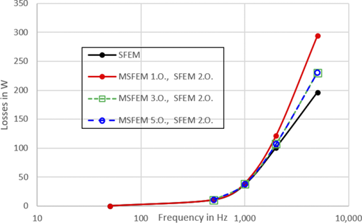
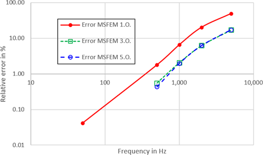
By adding higher-order terms, the accuracy is clearly improved. The reason why the fifth-order approach does not show a better accuracy than the third-order one is that the reference solution is not reliable for high frequencies. Reference solutions for an order higher than 3 could not be solved on the available server with 4 times 16 cores (Intel(R) Xeon(R) CPU E7-8867 v3) and 2 TByte RAM.
4.2 Time stepping method and time stepping method multiscale finite element method
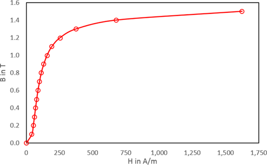
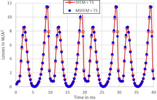
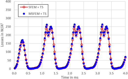
To deal with nonlinear materials simulations with the time stepping method (TSM) and MSFEM (TSMSFEM) have been carried out using implicit Euler as time stepping scheme and the fixed point method Bíró and Preis (1995) has been exploited to solve the nonlinear system. Iron is highly nonlinear, but assumed to be isotropic. The magnetization curve used in the simulations is determined by measurement points and linear interpolation (Figure 11). The curve is convex-concave. Input currents are selected with 1.0, 2.0 and 3.0 A (peak value) to deal with different states of saturation. Simulations with these currents have been carried out at 50 and 500 Hz. For the reasons of comparability, the eddy current losses in the laminated core presented in Figures 12 to 17 are scaled to the current in the wire of the coils I squared.
Scaled eddy current losses in Watt per Ampere squared versus time, f = 50 Hz and I = 1 A
Scaled eddy current losses in Watt per Ampere squared versus time, f = 50 Hz and I = 1 A
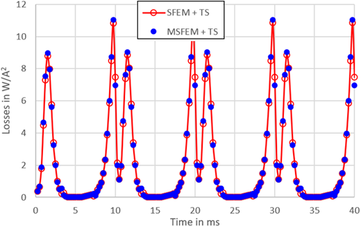
Scaled eddy current losses in Watt per Ampere squared versus time, f = 50Hz and I = 2 A
Scaled eddy current losses in Watt per Ampere squared versus time, f = 50Hz and I = 2 A
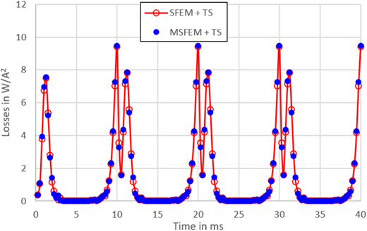
Scaled eddy current losses in Watt per Ampere squared versus time, f = 50 Hz and I = 3 A
Scaled eddy current losses in Watt per Ampere squared versus time, f = 50 Hz and I = 3 A
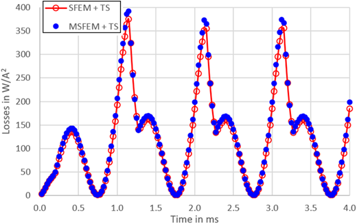
Scaled eddy current losses in Watt per Ampere squared versus time, f = 500 Hz and I = 1 A
Scaled eddy current losses in Watt per Ampere squared versus time, f = 500 Hz and I = 1 A
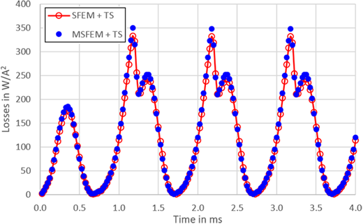
Scaled eddy current losses in Watt per Ampere squared versus time, f = 500 Hz and I = 2 A.
Scaled eddy current losses in Watt per Ampere squared versus time, f = 500 Hz and I = 2 A.
Scaled eddy current losses in Watt per Ampere squared versus time, f = 500 Hz and I = 3 A
Scaled eddy current losses in Watt per Ampere squared versus time, f = 500 Hz and I = 3 A
4.2.1 Results, 50 Hz.
The Figures 12 to 14 show the losses at f = 50 Hz. The agreement of the losses with respect to time obtained by SFEM and MSFEM is excellent. The influence of the saturation due to different input currents is clearly visible.
4.2.2 Results, 500 Hz.
Eddy current losses obtained at f = 500 Hz (Figures 15 to 17) show a clear transient initial phase behavior before the steady state is reached. A very satisfactory agreement between SFEM and MSFEM is obtained.
4.3 Harmonic balance method and MSFEM
Most of the sources of ECPs alternate harmonically in time and only the solution of the steady state has to be calculated. However, in case of nonlinear materials, the solution is not harmonic any more, but still periodic. Thus, the solution can be represented as a Fourier series. This can be exploited advantageously by the harmonic balance method (Yamada and Bessho, 1988) or as also called the multi-harmonic ansatz (Bachinger et al., 2005), i.e. a truncated Fourier series expansion at a finite number. Only a few harmonics are required for a sufficiently accurate approximation. That’s why the harmonic balance method is superior to the time stepping method particularly in case of a transient that takes a long time. The harmonic balance finite element method (HBFEM) saves mainly computation time in simulations of large devices with harmonic excitation and nonlinear material properties. A rigorous estimate for the total error due to the use of truncated Fourier series is presented in Bachinger et al. (2005). The successful use of HBFEM in simulations of electromagnetic devices in the frequency domain can be found in De Gersem et al. (2001) or in Gyselinck et al. (2002). A 2D FEM considering the main magnetic flux with a 1D diffusion equation across the lamination and using a multi-harmonic ansatz of the MVP including hysteresis is shown in Bottauscio et al. (2000).
The harmonic balance method is combined with the MSFEM (HBMSFEM) to exploit the advantages of both methods.
For nonlinear problems with time harmonic excitation and steady state, the harmonic balance method is preferably used (Bíró and Preis, 2006). The steady state solution u(x,t) is periodic in time with period T:
An approximated solution can be written as a truncated Fourier series:
with superscripts c and s for cosine and sine, respectively, and with the upper bound N.Based on the basic MSFEM approach [equation (4)], the HBMSFEM approach can be written as:
with the coefficient functions:
where α = c,s and k∈ℕ, k≤N holds. The time average A0(x) in equation (15) is not used in this work. The hat indicates truncated Fourier expansion of the HBMSFEM approach.
To compare the results of TS and HBFEM, the losses obtained by TS are averaged over the first and second period. Simulation results for the losses are summarized for f = 50 and f = 500 Hz in Appendix 1 in Tables I and II. There is a very satisfactory agreement.
Eddy current losses in W at f = 50 Hz
| I in A | 1 | 2 | 3 | |||
|---|---|---|---|---|---|---|
| Period \TS | SFEM | MSFEM | SFEM | MSFEM | SFEM | MSFEM |
| TSM 1st Period | 3.51 | 3.52 | 8.92 | 8.97 | 13.1 | 13.3 |
| TSM 2nd Period | 3.58 | 3.526 | 9.062 | 9.091 | 13.73 | 13.79 |
| HBMSFEMa | 3.979 | 9.112 | 14.05 | |||
Note:
Up to the 5th harmonic.
Eddy current losses in W at f = 500 Hz
| I in A | 1 | 2 | 3 | |||
|---|---|---|---|---|---|---|
| Period \TS | SFEM | MSFEM | SFEM | MSFEM | SFEM | MSFEM |
| TSM 1st Period | 104 | 108 | 401 | 412 | 632 | 646 |
| TSM 2nd Period | 135 | 141 | 537 | 550 | 853 | 869 |
| HBMSFEMa | 137 | 539 | 801 | |||
Note:
Up to the 5th harmonic.
5. Computational costs
The number of required degrees of freedom (DOFs) is valid for one-eighth of the single phase transformer and is given in Appendix 2 in Tables III. In general, using MSFEM the number of DOFs can be reduced by a factor of about ten for the studied example of the single phase transformer in the present work.
6. Discussion
The presented MSFEM fits very well to ECPs in transformers. Electrical machines can be treated in two ways. The assumption that each iron sheet is exposed to the same electromagnetic field pattern is often permitted. In this case, a 2D/1D MSFEM can be exploited advantageously (Schöbinger et al., 2019; Hollaus et al., 2018). However, when the stray field cannot be neglected or its influence is of interest, a method which copes with 3D problems is absolutely necessary. The presented MSFEM should also work for 3D problems of electrical machines.
The reduction of computational costs grows with the number of iron sheets in the laminated core. Although, applying MSFEM reduces large problems essentially, the remaining complexity is still too large to be solved conveniently. Further methods based on MSFEM needs to be developed.
Large equation systems resulting from problems with many very thin iron sheets compared to the overall dimensions of the core are extremely ill-conditioned and except small problems impossible to solve iteratively due to the lack of an appropriate preconditioner. Similarly, an appropriate preconditioner is missing for equation systems from the MSFEM too. Therefore, both the reference problems and the MSFEM problems have been solved using a direct solver.
7. Conclusions
Based on the results in this work, it can be concluded that the MSFEM presented here is very powerful because it reduces the complexity of the ECP in laminated iron cores essentially compared to SFEM and discretizing each sheet, copes with any penetration depth, considers the edge effect, allows to include nonlinear material properties in a straightforward way and is capable to deal with real 3D problems.
This work was supported by the Austrian Science Fund (FWF) under Project P 27028.

