
This paper aims to model a three-dimensional twisted geometry of a twisted pair studied in an electrostatic approximation using only two-dimensional (2D) finite elements.
The proposed method is based on the reformulation of the weak formulation of the electrostatics problem to deal with twisted geometries only in 2D.
The method is based on a change of coordinates and enables a faster computational time as well as a high accuracy.
The effectiveness of the adopted approach is demonstrated by studying different configurations related to the IEC 60851-5 standard defined for the measurement of the electrical properties of the insulation of the winding wires used in electrical machines.
1. Introduction
Using twisted wires in electrical engineering goes back to the late 19th century, when Bell introduced them to mitigate the crosstalk between the first telephone and a telegraph (Bell, 1876). They soon became commonplace in many electric and electronic applications and are in particular used as a means to test the aging of the insulation of electrical machines (Guastavino and Dardano, 2012) and to extract the electrical properties of their insulation (IEC, 2019).
Several studies have investigated the effect of twisted wires on the surrounding environment (Moser and Spencer, 1968), a nearby single wire (Paul and Jolly, 1982) or the ground (Pignari and Spadacini, 2011), by using predictive models. However, the accurate calculation of the distributed capacitances or the local electromagnetic fields, e.g. the local electric field strength for realistic configurations, requires costly three-dimensional (3D) simulations (Acero et al., 2014; Lyly et al., 2012). While a method based on several two-dimensional (2D) simulations (on slices of the 3D geometry) was proposed in Gustavsen et al. (2009), it introduces an intrinsic modeling error because of the performed averaging and cannot recover the true 3D local fields.
In this paper, following the approach originally derived in Nicolet et al. (2006, 2007a), we propose to reformulate the 3D problem in helicoidal instead of Cartesian coordinates (Waldron, 1958), leading to a 2D formulation with an adapted metric, easy to implement in existing 2D finite element codes. For purely helicoidal and infinitely long 3D geometries, the proposed 2D formulation is exact. The gains are twofold: the geometrical modeling and meshing of the potentially complex multi-layer conductors usually with large aspect ratios can be performed on a 2D slice instead of in 3D; and the finite element solution is greatly reduced.
The paper is organized as follows. After describing the geometrical configuration of twisted pairs in Section 2, the 3D electrostatic problem is reformulated in helicoidal coordinates in Section 3, leading to a 2D finite element formulation with an adapted metric – the “2D twisted” model. This 2D twisted model is verified against the full 3D model in Section 4 by computing the conductor charges in function of the number of turns in a twisted pair of enameled wires. Next, the improvement in accuracy of the 2D twisted model compared to the usual 2D (straight) model is analyzed in Section 5 in function of the number of turns, the conductor diameter and the insulation thickness. The effectiveness of the approach is finally demonstrated by studying different configurations related to the IEC 60851-5 standard for the measurement of the electrical properties of winding wires.
2. Geometry of twisted wires
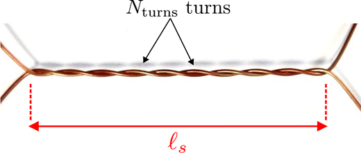
The twisted geometry is defined by a number of turns Nturns over a swirl length ℓs (Figure 1). One spatial period of the twisted pair is depicted in Figure 2, where the extrusion length ℓe (i.e. the linear length of the spatial period) and the length of the helix ℓh (i.e. the length of the mean fiber of each twisted conductor) are defined as follows:
with d and ℓi being the diameter of the conductors and the insulation thickness, respectively. Finally, the torsion of the twisted pair is defined as .
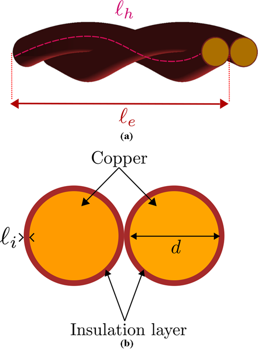
(a) One spatial period of the twisted pair. (b) The geometrical parameters of the cross-section
(a) One spatial period of the twisted pair. (b) The geometrical parameters of the cross-section
3. Twisted electrostatic model
To study the capacitive coupling between the twisted wires using the finite element method, we first derive a weak form of Maxwell’s equations in the electrostatic approximation.
3.1 Electrostatic model
Assuming zero free charge density, and denoting the (static) electric field and the dielectric permittivity in Cartesian coordinates (x1, x2, x3), respectively, by e(x1, x2, x3) and ε(x1, x2, x3), Maxwell’s equations reduce to:
where curlx and divx are the classical curl and divergence operators in the Cartesian coordinates system, respectively. Defining the scalar electric potential v(x1, x2, x3) such that e = −gradx(v), (2) leads to the second-order equation as follows:
where gradx denotes the gradient operator in Cartesian coordinates.
Our aim is to solve (3) in a domain Ωx enclosing the twisted pair, with a prescribed scalar potential on the (boundary of the) conductors. To use the finite element method, Ωx is bounded and an appropriate geometrical transformation is defined in an annular region to handle the natural extension of fields to infinity (Henrotte et al., 1999; Remacle et al., 1994; Bossavit, 1998). The annular region (of inner and outer radii Rint and Rout, respectively) is depicted in Figure 3. The boundary ∂ Ωx of Ωx is thus composed of the boundary of the conductors in the twisted pair Γc and the outside boundary of the annular region Γout.
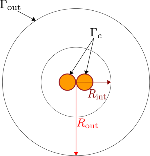
Bounded domain with annular region with geometrical transformation to handle the natural extension of fields to infinity
Bounded domain with annular region with geometrical transformation to handle the natural extension of fields to infinity
3.2 Weak formulation in Cartesian coordinates
Let us assume that the potential v is fixed to zero on Γout and to a prescribed value vc(x1, x2, x3) on Γc. The weak formulation of (3) writes (Ern and Guermond, 2013): find v ∈ H1(Ωx) with v = vc on Γc and v = 0 on Γout, such that:
holds for all test functions . Here, H1(Ωx) denotes the classical Sobolev space on Ωx, and its subspace with functions vanishing on the boundary ∂ Ωx. For the 3D geometry, periodic boundary conditions along the x3 axis are used. After discretizing Ωx with a finite element mesh, and choosing suitable finite dimensional subspaces (e.g. with piecewise linear or quadratic shape functions), (4) becomes:
where the superscript “T” denotes the transpose, whereas vh and denote the finite dimensional approximation of v and v′, respectively, leading thus to the classical matrix system.
Following the approach described in Nicolet et al. (2006, 2007a), we now reformulate the weak formulation (5) in helicoidal coordinates.
3.3 Helicoidal coordinates
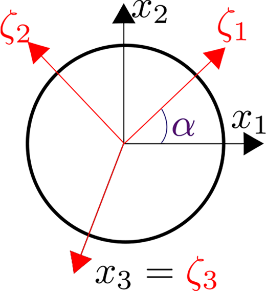
Helicoidal coordinates (ζ1, ζ2, ζ3) are related to the Cartesian coordinates (x1, x2, x3) through the following relations (Figure 4) (Waldron, 1958):
or, conversely:
The Jacobian of the transformation from helicoidal to Cartesian coordinates is defined as follows:
which, using (6), writes:
If gradζ denotes the gradient in helicoidal coordinates and J−T the inverse of the transpose of J, we have:
and the weak form (5) in helicoidal coordinates becomes (because dΩx = det(J)dΩζ: find vh such that:
where Ωζ refers to the domain of study in helicoidal coordinates. Equation (11) can be further simplified as follows:
with T−1 the symmetric matrix:
thus making (12) become:
Formally, comparing (5) to (14), the dielectric material represented by the scalar permittivity ε in Cartesian coordinates is thus replaced in helicoidal coordinates by an equivalent anisotropic and inhomogeneous permittivity tensor density εT−1 (Nicolet et al., 2007a, 2007b). The matrix T−1(ζ1,ζ2) being independent of ζ3, (14) can be reduced to a 2D problem in terms of coordinates ζ1 and ζ2, on a “slice” of the 3D geometry with constant ζ3 = x3, without information loss. When expressed in polar coordinates (ρ,ϕ) defined as follows:
with can be rewritten as follows:
where R(ϕ) is the rotation matrix:
As mentioned in Section 3.1, the domain of study is bounded by an annular region of inner and outer radii Rint and Rout, respectively, to handle the natural extension of fields to infinity. The matrix is thus piecewise defined, with (16) being valid for ρ ≤ Rint. The expression of the matrix for ρ ∈ ]Rint, Rout] is presented next.
3.4 Infinite transformation
In the annular region ρ ∈ ]Rint, Rout], a geometrical transformation is applied to handle the natural extension of the fields to infinity (Henrotte et al., 1999; Remacle et al., 1994), and the matrix T−1 writes:
The parameters r and dr are the transformed radial cylindrical coordinates and the derivative of r, respectively:
The infinite transformation can be seen as a change in the physical properties of the “infinite air,” thus an anisotropic and piecewise defined tensorial permittivity is used in the 2D finite element implementation.
4. Verification of the two-dimensional twisted model
Given the spatial periodicity of the geometry, only one spatial period referred to as the 3D geometry, with its cross section defining the 2D geometry is studied. For all geometries, created and meshed using Gmsh (Geuzaine and Remacle, 2009), an “infinite” transformation is applied in an annular region as described in Section 3.4. The 3D geometry was used to solve (5) and the 2D to solve (14). The finite element computations were performed using the open source finite element solver GetDP (Dular et al., 1998a).
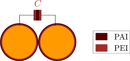
In real applications, enameled conductors are coated in successive thin layers to ensure correct polymerization and cross-linking. This defines the thermal and electrical performance of the wire. A classical arrangement is polyester-imide (PEI) as the first layer and polyamide-imide (PAI) on top. Additionally, for this case study the layers were given the same thickness. Thus, ε is defined as a piecewise function and its values were chosen for the two layers in 3D to be εPEI = 4.5ε0 and εPAI = 2.4ε0, where F m−1 is the vacuum permittivity, 4.5 and 2.4 being the relative permittivities of PEI and PAI, respectively. The equivalent anisotropic and inhomogeneous dielectric permittivity for the 2D twisted study is hence easily deduced (Section 3.3). This is portrayed in Figure 5, where a capacitor is used to illustrate the capacitive coupling between the two conductors.
To verify the 2D twisted model, simulations were run where the quantity of interest is the charge per meter Q of the system (Dular et al., 1998b). Using finite elements, and for both geometries, the computation of the charges per meter is done as follows:
where n is the outside normal to Γc, Q3D is the charge computed in 3D converted to a 2D value by dividing by ℓe and is the charge computed by the 2D twisted model.
Finite element computations were performed for a predefined range of Nturns per meter varying from 64 to 768, for a fixed value of ℓs. In all computations the potential difference between the two conductors was set to 1 V, and the potential at infinity was set to 0 V. The results are presented in Figure 6, where the corresponding 3D geometries were added to illustrate the amount of twist. The relative error used for comparison is defined as follows:
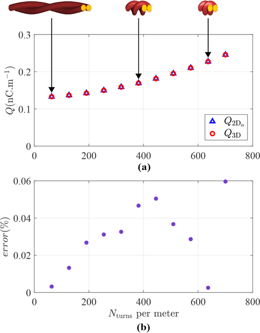
(a) Comparison of the computed charges per meter for the 2D and 3D geometries. (b) The relative error between Q3D and
(a) Comparison of the computed charges per meter for the 2D and 3D geometries. (b) The relative error between Q3D and
As depicted in Figure 6(b), the relative error does not exceed 0.06%, which validates the twisted model. (The remaining small error is because of the small discrepancy between the 3D mesh and the exact twisted geometry.) The computational efficiency of the 3D and 2D models is reported in Table 1. The number of nodes in the 3D mesh is about 21 times the number of nodes in 2D mesh, which explains the large difference in the computational times: 16 min for the 3D model and only 8 s for the 2D model.
Comparison of the computational efficiencies of the 2D and 3D models
| 2D | 3D | |
|---|---|---|
| No. of nodes | 47,755 | 1,002,945 |
| No. of elements | 101,188 | 2,226,182 |
| Computational time | 8 s | 16 min |
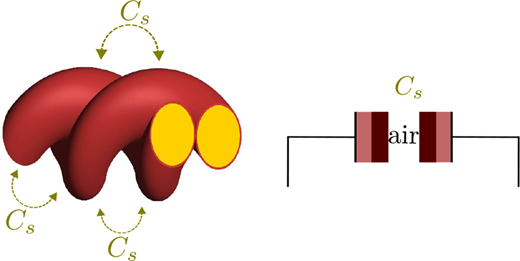
As noticed in Figure 6(a), the increase of Nturns yields an increase in the computed charge, which is because of the increase of the capacitive coupling between the different parts of the studied conductor. This extra capacity, referred to as Cs, is illustrated in Figure 7. The higher Nturns, the less air there is between the two electrodes of the equivalent capacitance Cs, the higher is the computed charge. It is also worth mentioning that for very high and non-physical values of Nturns, the relative error starts to increase, because of the increased deformation of the 3D mesh. Finally, it should also be noted that in addition to global quantities like the charge, the 2D model also allows to retrieve local quantities like the electric field strength.
5. Impact of the twisted geometry on the computed values
To emphasize the importance of using the proposed 2D twisted model instead of simplifying the study to a 2D straight model, we study the influence of the geometrical parameters Nturns, d and, ℓi over the computed charges and . The latter is the computed 2D charge for a straight geometry, i.e. with α = 0.
5.1 Impact of the number of turns
To study the impact of the number of turns Nturns over the computed 2D charges, d was fixed to 0.8 mm, and ℓi to 28 µm. A new variable is introduced corresponding to a corrected 2D twisted 2D charge deduced from a straight charge analytically, as follows:
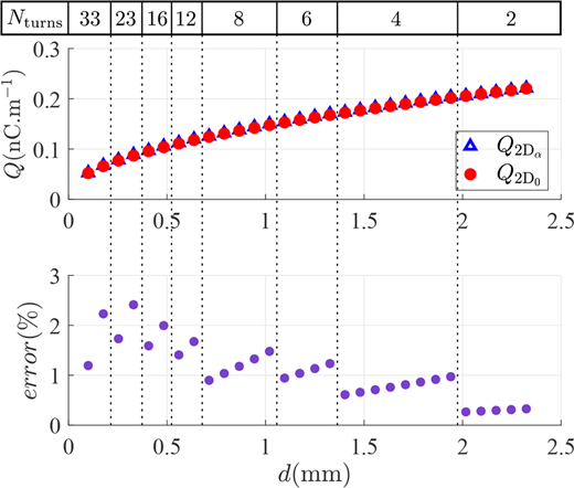
where ℓe and ℓh are defined in Figure 2. The results are plotted in Figure 8, where error1 and error2 are computed as in (21):
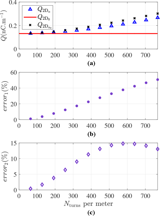
(a) Study of the impact of the number of turns per meter on and . (b) The computed relative error between and . (c) The computed relative error between and
(a) Study of the impact of the number of turns per meter on and . (b) The computed relative error between and . (c) The computed relative error between and
The higher the value of Nturns, the higher , whereas remains constant because no twist is geometrically introduced. For Nturns per meter equal to 64, the relative error is roughly 1.0549% and increases with Nturns because of the emergence of new capacitive coupling as elaborated in the previous section, increasing thus the discrepancy between the two.
The engineering approach adopted to correct the 2D straight values to twisted ones thus gives approximate, but not precise, values of the twisted charges. Therefore, the ratio of lengths is not enough to compute the value of the twisted charge. This proves the added value of the 2D twisted model and the importance of its usage when it comes to a twisted geometry. Indeed, the proposed 2D twisted model has the same computational efficiency as the 2D straight model, does not need a post processing (i.e. correcting the straight values with the length ratio) and fully considers the impact of the twist over the computed values.
5.2 Impact of the diameter of the conductor
To study the impact of the diameter of the conductor, Nturns per meter was set to 320 turns and ℓi to 28 µm. The diameter was varied from 0.4 to 5.16 mm. The results are seen in Figure 9.
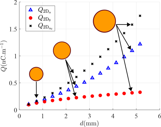
As expected, the charges, straight and twisted, increase with the diameter of the conductor because the surface of the copper increases as well. This is illustrated in Figure. 5 and even though the two conductors are not planar, the formula for plane capacitors can be used to understand the impact:
where A is the surface of the parallel copper plates, which increases with d. Moreover, the two charges and do not increase in the same manner. This is seen in Figure 7, where the twisted geometry introduces capacitive coupling between the different parts of the twisted conductors (Cs): the higher α, the lesser the thickness of the equivalent insulation of Cs, the higher is the value of the computed charge. The values of were also computed and plotted in Figure 9, where the discrepancy between and is because of the increase of the values of d, which increases the value of the length ratio (ℓh increases with d, whereas ℓe is constant because Nturns is constant).
5.3 Impact of the insulation thickness
Here, d was set to 0.8 mm and Nturns per meter to 320. The insulation thickness ℓi was varied from 10 to 50 µm. The results are seen in Figure 10 where a 2D geometry is presented to visualize the impact.
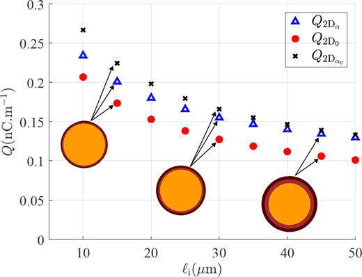
Following the same explanatory approach used in Section 5.2, and by making use of the parallel plate capacitive coupling analogy, the results can be easily interpreted as well. The capacitance (or the charge because ΔV = 1 V) is inversely proportional to the thickness of the dielectric. Thus, the smaller ℓi, the easier the storage of the charges. For this study also, the values of were computed and seem to converge to for very high non-physical values of ℓi.
5.4 Study of the standard IEC 60851-5
As an application to the developed model, we propose to investigate the twist configurations in the IEC 60581-5 standard (IEC, 2019), which are summarized in Table 2.
IEC 60581-5 Standard
| Range of the diameter (mm) | Nturns | Nturns per meter |
|---|---|---|
| 0.100 ≤ d < 0.250 | 33 | 246 |
| 0.250 ≤ d < 0.355 | 23 | 184 |
| 0.355 ≤ d < 0.500 | 16 | 128 |
| 0.500 ≤ d < 0.710 | 12 | 96 |
| 0.710 ≤ d < 1.060 | 8 | 64 |
| 1.060 ≤ d < 1.400 | 6 | 48 |
| 1.400 ≤ d < 2.000 | 4 | 32 |
| 2.000 ≤ d < 2.500 | 2 | 16 |
For each diameter range d, a value of Nturns (ultimately α) is defined for ℓs = 0.125 m, which is also fixed by the standard. The higher the value of d, the lesser the Nturns and the less twisted the geometry is. The performed study consists in computing for each d varying from 0.1 to 2.4 mm, ultimately the upper and lower bounds of the specified range, the 2D charges: and . Their variations according to d are plotted in Figure 11. The relative error was computed as in (21) (i.e. error1). Here, the maximum number of turns Nturns per meter does not exceed 264 turn per meter (value computed for Nturns = 33) which is inferior to the values chosen in Sections 5.1–5.3.
In Figure 11, two parameters vary: the diameter d and the number of turns Nturns. To understand the variations, each sub-range where only one parameter varies will be studied separately. Taking, for instance, the sub-range of d where Nturns = 4, corresponding to a diameter varying between 1.4 and 2 mm, increasing d increases simultaneously the charges (, ) as well as the relative error between the two. This agrees well with the results of Section 5.2. Moreover, the variation of the slope of the relative error is because of the decrease of Nturns with the increase of the value of d. The higher the d is, the less twisted the geometry is, the smaller the value of Cs, the slighter is the difference between the twisted and straight charges until it eventually nullifies for a Nturns = 0. It should also be mentioned that in real applications, the insulation thickness ℓi also varies with the diameter d (IEC, 2013) which was considered constant for the study of the standard.
6. Conclusion
This paper presents an efficient method to solve a 3D twisted electrostatic problem using 2D finite elements based on a helicoidal change of coordinates. The object of study is a twisted pair widely used in different electrical engineering applications. The low time complexity of the 2D model is highlighted, as well as its high accuracy, when compared to the 3D model. The importance of using a 2D twisted geometry instead of a 2D straight geometry to study a 3D twisted problem is emphasized.
The proposed model, by inserting the correct permittivities of the dielectric materials used in real application, could efficiently provide the value of the capacitance between twisted wires. The model may even be used as an alternative to measurements, enabling the analysis of twisted wires only by simulations. The model could also be adopted for various other case studies of twisted pairs: a Debye model could, for example, be used to describe the frequency-dependent behavior of the used insulation; or the impact of the temperature over the permittivity that could also be taken into account by using, e.g. an Arrhenius model.
This work is co-financed by the European Union with the financial support of European Regional Development Fund (ERDF), French State and the French Region of Hauts-de-France.
