
Nonlinear solution approaches for inverse problems require fast simulation techniques for the underlying sensing problem. In this work, the authors investigate finite element (FE) based sensor simulations for the inverse problem of electrical capacitance tomography. Two known computational bottlenecks are the assembly of the FE equation system as well as the computation of the Jacobian. Here, existing computation techniques like adjoint field approaches require additional simulations. This paper aims to present fast numerical techniques for the sensor simulation and computations with the Jacobian matrix.
For the FE equation system, a solution strategy based on Green’s functions is derived. Its relation to the solution of a standard FE formulation is discussed. A fast stiffness matrix assembly based on an eigenvector decomposition is shown. Based on the properties of the Green’s functions, Jacobian operations are derived, which allow the computation of matrix vector products with the Jacobian for free, i.e. no additional solves are required. This is demonstrated by a Broyden–Fletcher–Goldfarb–Shanno-based image reconstruction algorithm.
MATLAB-based time measurements of the new methods show a significant acceleration for all calculation steps compared to reference implementations with standard methods. E.g. for the Jacobian operations, improvement factors of well over 100 could be found.
The paper shows new methods for solving known computational tasks for solving inverse problems. A particular advantage is the coherent derivation and elaboration of the results. The approaches can also be applicable to other inverse problems.
1. Introduction
The inverse problem of electrical capacitance tomography (ECT) is to determine the spatial relative dielectric permittivity distribution εr(x, y) in a domain ΩROI (region of interest) based on capacitive measurements (Neumayer et al., 2011, 2012). Figure 1 depicts a 2D scheme of an ECT sensor for process tomography, where the sensing principle is applied to monitor material distributions inside pipes or vessels. The region ΩROI is the interior of a nonconductive pipe/vessel. Nelec electrodes are attached to the outside of the tube. The measurements are given by the M = Nelec(Nelec–1) inter electrode capacitances. To obtain these measurements, an alternating current voltage is applied to one electrode. This electrode is referred to as the active electrode. At the other electrodes, the displacement currents to ground are measured, which are proportional to the inter electrode capacitances. This process is repeated for each electrode. To improve the immunity against external influences, the sensor is shielded by a screen that is connected to the ground potential.
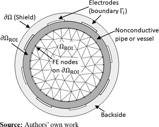
The solution of the inverse problem of ECT then requires a model for the description of the material distribution εr(x, y) and a forward model for the simulation of the measurements (Kaipio and Somersalo, 2004). The domain within the shield is denoted by Ω. ∂Ω denotes its boundary, and Γi, i = 1, …, Nelec, denotes the boundaries of the electrodes. The governing partial differential equation (PDE) for ECT within Ω is given by ▽·(εr▽V) = 0, where V is the electric scalar potential. In the sensor simulation, the PDE is solved according to the measurement process. The boundary conditions on all electrodes and the shield are of Dirichlet type with on the active electrode and V = 0 on all other boundaries. Given the solution Vi for the ith electrode being the active electrode, the measurements are evaluated by (j = 1,…, Nelec, j ≠ i). The results of the integral evaluation are stored in the Nelec × Nelec matrix Q. Hence, the simulation of the measurement requires Nelec solving the PDE. Note that, actually, only M/2 independent measurements can be made due to the reciprocity property. Also, note that, we compute charges as simulated measurements, as we skip a normalization by V0. Yet this is no issue for our further discussion. In measurement applications, a calibration is performed between the sensor and the simulation model. The calibration compensates for affine deviations between the sensor and the model (Neumayer et al., 2011); hence, it comprises the strength of the excitation signal.
Throughout this work, we will use the finite element (FE) method for the simulation of the sensor and the description of the material distribution εr(x, y). Following Figure 1, the spatial permittivity distribution εr(x, y) is modeled by means of the FE discretization in ΩROI forming the vector εr ∈ RN. The simulation of the sensor is given by the FE equation system:
where is the symmetric NFEM × NFEM stiffness matrix. The NFEM × NElec matrix R holds the right-hand side vectors for the excitation pattern of the measurements. For the incorporation of the boundary conditions in the matrix , we use the scheme of keeping the essential nodes (Ern and Guermond, 2004). The matrix V is of the same dimension as the matrix R, its column vectors hold the corresponding solution vectors for the scalar potential. Thus, equation (1) comprises all NElec solves. It is important to point out that the matrix is linear with respect to the elements of εr due to the FE matrix assembly scheme (Ern and Guermond, 2004). The computation of Q is given by (Yan et al., 1998):
where we refer to the sparse NElec × NFEM matrix M as measurement matrix. Its nonzero coefficients represent the integral evaluation discussed in the previous paragraph. Note that equation (2) also provides the diagonal elements of Q. In our work, the matrix M is constant. So are the elements of which represent the pipe and the backside of the ECT sensor.
Recent publications present a significant potential for the application of ECT technology for flow monitoring and mass flow metering in pneumatic conveying (Suppan et al., 2021; Suppan et al., 2019, 2022; Neumayer et al., 2019a, 2019b, 2017). Also, applications in environmental sensing (Bretterklieber et al., 2016; Flatscher et al., 2017, 2015) and safety applications have been addressed (Fletcher, 1987). A prerequisite for these applications is the ability for fast numerical simulation techniques for the sensor. This does not only comprise the solution of equation (1) where the assembly of is a known bottleneck but also computations involving the M × N Jacobian matrix (i = 1,…, M, j = 1,…, N). This is relevant for optimization based inverse problems methods, e.g. the gradient g ∈ RN of the objective function can be evaluated by g = JTΔq, with Δq = q(εr)–qmeas being the residual vector (Neumayer et al., 2019c). Here, q ∈ RM is a vector holding the measurements. In statistical inversion theory, the Jacobian is used as an approximation of the form JΔεr to speed up Markov chain Monte Carlo methods (Watzenig et al., 2011; Brandstatter, 2003).
The computation of the Jacobian has been addressed by several researchers. Two common techniques are the adjoint field method (Bradley, 2013; Brančík, 2004) and techniques based on the derivation of the stiffness matrix (Adler et al., 2017; Young, 1988), whereby in (Young, 1988) also an equivalence between these methods is addressed. For the computation of the Jacobian using adjoint field methods, an additional equation system of the form of equation (1) has to be solved (Bradley, 2013). This makes the calculation of the Jacobi expensive, especially since we are interested in matrix vector products of the Jacobian or its transpose.
In this work, we present fast numerical techniques for the addressed computational bottlenecks. In particular, we will show that matrix vector products including the Jacobian or its transpose can be computed for free, i.e. without any additional solves. The contributions and novelty of the paper are:
a solution approach based on Green’s functions;
fast stiffness matrix assembly technique based on an eigenvector decomposition;
Jacobian operations to evaluate JΔεr and JTΔq without an explicit evaluation of the Jacobian; and
demonstration of methods the within a BFGS (Broyden–Fletcher–Goldfarb–Shanno)based Gauss Newton scheme for deterministic inversion.
The methods include dedicated pre-processing steps as well as techniques, which are used during the solution of inverse problems. In the following sections, we address these points.
2. Solution with Green functions
In this section, we present the solution of equations (1) and (2) by a Green’s functions approach and a modified charge computation scheme. Note that, the later scheme is not required but offers some further options, which we will address.
As depicted in Figure 1, only the material values in the domain ΩROI change. The properties (geometry and material values) of the domain do not change. We therefore propose a charge computation scheme of the form:
The computation of the charges is therefore based on potential of the FE nodes on the boundary ∂ΩROI, which is the inner wall of the tube. The charge matrix represents the “sensor backside.” has the same dimensions as the matrix Q, and has the dimension of . Both matrices can be determined numerically. For the determination of , a sensor simulation is performed, where the potential on ∂ΩROI is set to zero. The elements of are determined by simulations where the potential on each node is set to one, while all other nodes have the potential of zero. The addressed computations are carried out in a preprocessing step.
Based on equation (3), the evaluation of Q now requires the evaluation of the potentials on ∂ΩROI, which are held in the matrix . Instead of assembling from V by solving (1), we take advantage of the symmetry of , which allows the computation of by:
The matrix holds the identity vectors corresponding to the FE node numbers for the nodes on ∂ΩROI. The column vectors of G are referred to as Green’s functions (Zhang and Fuzhen, 2005). From equation (5), it can be seen that Green’s functions act as an” inverse operator”, i.e. it can be used to replace . This property will be used for the later addressed methods. Yet equation (4) has a significant disadvantage as simulations are required. We therefore right multiply equation (4) with , which yields to:
and:
for the evaluation of the charges. Solving equation (6) for GQ and computing the charges Q by (7) requires the same computational effort as the original problem, i.e. equations (1) and (2).
2.1 Comment on the choice of the charge computation
The evaluation of Q based on the potential as shown in equation (3) is based on the property that only the material within the domain ΩROI changes. Yet this choice for the charge computation is not unique. E.g. also from the nonzero columns of M in equation (2), a charge computation scheme can be derived. The Green’s functions then have to be computed for the corresponding FE nodes, and the remaining scheme is the same as discussed above. However, we would like to point out that by using for the charge calculation, further possibilities for the solution of (6) arise. E.g. as only the block matrix corresponding to ΩROI within changes, the Schur complement (Strang, 1986) might be used for its solution. We have not investigated this further in this work but want to make a note on it in relation to the choice of equation (3).
2.2 Properties of GQ
The computation of GQ in equation (6) offers significant advantages in conjunction with evaluations including the Jacobian matrix J. This will be addressed in Section 4 and is due to two properties:
The Green’s functions GQ can be used to replace the product term ; and
For the FE nodes in ΩROI, the Green’s functions GQ equal the negative solution for the scalar potential V, i.e. GQ = –V holds in ΩROI.
The first property can be seen from equations (3) and (5).
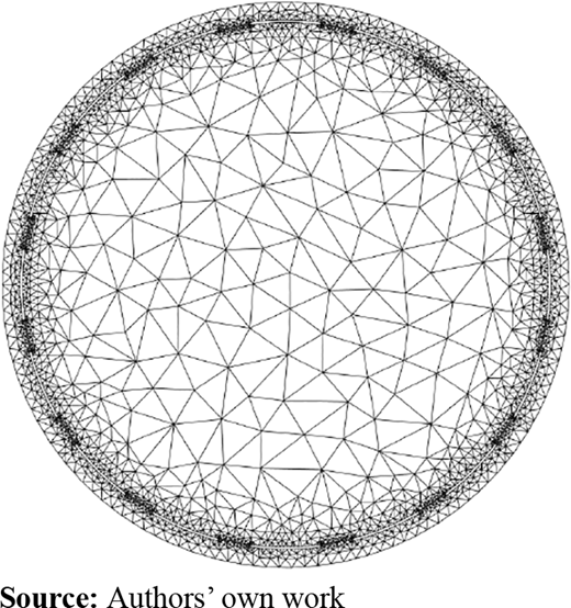
The second property is less obvious but can be found from an analysis of the right-hand side matrices R and RQ. For the sake of the length of this derivation, we want to show a numerical result here. Figure 2 depicts a 2D FE mesh of an ECT sensor with Nelec = 16 electrodes. The mesh has about 5,000 elements and about 3,000 FE nodes. The number of FEs in ΩROI (N) is about 700. The field plots in Figure 3 depict a column of V (left), GQ (center) and the difference (V–GQ) (right) for a 2D FEM simulation of an ECT sensor, respectively. For the FE nodes in ΩROI, the scalar potential V equals –GQ. Hence, we can replace V by –GQ for computations involving the domain ΩROI. This will be shown in Section 4.1.
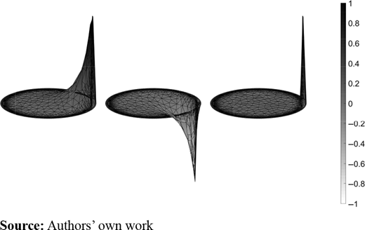
Exemplary visualization of a column of V (left), GQ (center) and the difference V–GQ (right) for a 2D FEM simulation of an ECT sensor. Within the domain ΩROI, the solution V equals –GQ
Exemplary visualization of a column of V (left), GQ (center) and the difference V–GQ (right) for a 2D FEM simulation of an ECT sensor. Within the domain ΩROI, the solution V equals –GQ
3. A fast matrix assembly scheme based on an eigenvector decomposition
A commonly known bottleneck in FE simulations is the assembly of the stiffness matrix. While this is less of an issue for single simulations, it can become a significant issue for the solution of inverse problems due to the required repeated simulation process. A well-known technique is to reduce the assembly effort by splitting into a constant part and a variable part which is changed, e.g. as , where Ke,i are the FE element matrices. Here, the linearity of with respect to the elements of εr can be seen. Yet the implementation of the update term can still remain a bottleneck, e.g. a loop type implementation without memory allocation is not suitable here.
Numerical linear algebra routines are highly efficient in the evaluation and storage of vector products of the form abT or matrix products of the form ABT. Note that these products create matrices. For our further discussion, we use FEs of the order p = 3, i.e. the element matrices Ke,i are of the form Ke = [ke,1 ke,2 ke,3], where the vectors ke,i are its column vectors. Using these vectors, the element matrix can be expressed by .
We can expand this scheme by placing the column vectors ke,i within the sparse NFE × N matrices such that the elements of ke,i appear at their global node number. Then the FE equation system can be assembled by:
where hold the required identity vectors. This scheme, in conjunction with linear algebra routines, is already a highly efficient assembly technique for .
A further improvement can be obtained by exploiting the symmetry and positive semi-definiteness of the element matrices. For the exemplary case of p = 3, the eigen-decomposition provides:
where the vectors vi are its eigenvectors and di are the corresponding positive eigenvalues. As one eigenvalue is zero, the decomposition can be written as:
By defining , we can therefore assembly Ke by . Hence, at the cost of an eigenvector decomposition in the pre-processing phase, we can reduce the sum in the assembly process to p – 1, which corresponds to a reduction of one third for linear triangular elements.
By storing the vectors ai in the NFE × N matrices as addressed before, the stiffness matrix assembly can be performed by:
The presented decomposition is known in literature as a ATCA decomposition (Hansen, 1998) that can be applied to equilibrium systems. Note that the transpose operation appears in the first matrix of the ATCA decomposition, whereas in our derivation it appears in the last matrix. For our derivation, this is due to the notation of the eigenvector decomposition. Here, a change of the transpose sign can be seen as a definition.
3.1 Timing measurements for equation (12)
To evaluate the performance, we performed timing measurements of our MATLAB implementation using MATLABs profiler function. For the FE mesh depicted in Figure 2, we achieved an average execution time for equation (12) of 58 μs on an AMD Ryzen 5 2500U processor. In contrast, a (naive) loop implementation lasted several 10 ms. The average overall time to compute the charges is 9 ms. It should be noted that the presented calculation schemes also provide the possibility of parallelization.
4. Jacobian operations
In this section, we present the efficient evaluation of matrix vector products JΔεr and JTΔq, where J is the M × N Jacobian matrix.
4.1 Fast evaluation of JΔεr
We first study the derivation with the expression:
which expresses the deviation of the potential V by dV due to a change of the FE stiffness matrix by dK. Here again, the linearity of is applied. From the product , we obtain:
The differential change of the scalar potential is therefore:
and due to equation (2), we can also write:
By this, a derivative of Q with respect to the εr,i can be expressed by:
The elements of in equation (17) therefore provide the rows of the Jacobian J. gives the element matrix of the corresponding FE. Note that has the same dimension as the original FE equation system. Due to the linearity, we can therefore express JΔεr by
Equation (18) provides a Jacobian operation, i.e. an evaluation of the matrix vector product without an explicit evaluation of J but at the cost of solving Nelec equation systems with the stiffness matrix . We can know take advantage of the properties of the Green’s functions GQ. The product can be directly replaced by . Since only leads to matrix entries for the domain ΩROI, we can replace V by –GQ. Thus, we obtain
i.e. a Jacobian operation that can be directly computed from the solution of equation (6).
The inner matrix can be assembled by any desired scheme, yet because of its advantage, we propose the use of the eigenvector-based assembly technique addressed in Section 3, which leads to:
4.2 Fast evaluation of JTΔq
The derivation of a fast evaluation of JTΔq based on the use of the Green’s function is unfortunately not as straight forward as the derivation of JΔεr shown in Section 4.1. The derivation is based on studying the transpose of equation (19) for the column vectors of the matrix V. Furthermore, a matrix decomposition for the form ABT is required for the element matrices. This equals the discussion in Section 3. Because of the length, we will therefore only state the final result using the eigenvector-based stiffness matrix assembly. The evaluation of JTΔq can be performed by:
where ⊙ denotes a row- and column-wise multiplication. The matrix ΔQ is assembled from the residual vector Δq following the measurement scheme. Elements of Q that are not used for measurements are set to zero. Hence also the matrix vector product JTΔq can be directly evaluated given GQ, i.e. after the solution of equation (6).
4.3 Timing measurements for equations (20) and (21)
We again performed timing measurements for our implementation, where we achieved average execution times for equation (20) of 0.8 ms. The computation setup is the same as discussed in Section 3.1. We also performed timing measurements with a reference implementation of an adjoint field method (Bradley, 2013), which lasted about 350 ms. This comparison is not entirely fair, as the implementation of the reference method was not fully optimized. Yet it is relevant that the evaluation of equations (20) and (21) does not require any additional solves. We found a second comparison by comparing the evaluation of equation (20) against the evaluation of JΔεr when the Jacobian J is given. The evaluation of JΔεr last on average 0.2 ms. The factor of four between these times is in favor of equation (20), since it does not require an explicit evaluation of J. Timing tests for the evaluation of equation (21) lead to similar results.
5. Application of JTΔq within a Broyden–Fletcher–Goldfarb–Shanno based Gauss Newton scheme
The presented numerical techniques are intended to speed up the solution of inverse problems, i.e. the reconstruction of the material distribution εr from measurements qmeas. In this section, we demonstrate this by means of an exemplary reconstruction example where we estimate εr using the deterministic approach:
The first term in the objective function fits the model against the measurement. The second term is a regularization term, which is necessary due to the ill-posed nature of the inverse problem. For the matrix L, we used as second order derivative operator, which leads to a smoothing of the reconstruction result (Neumayer et al., 2011). The regularization parameter α was selected using the L-curve criterion (Hansen, 1998). For the solution of Adler et al. (2017), we use the Gauss–Newton method to compute a descent direction by , where Hk is the Hessian and gk is the gradient of the objective function. Here, we use the BFGS approximation of the inverse Hessian (Neumayer et al., 2019c). The algorithm is given by:
evaluate the Newton direction ;
set εr,k+1 = εr,k + spk and set sk = spk;
compute zk = g(εr,k+1) – g(εr,k+1); and
evaluate .
The gradient gk is the sum of the gradient of and the gradient of the regularization term. The first component is evaluated by equation (21), which requires one computation of the Green’s functions GQ. The gradient of the regularization term can be computed analytically. The variable s in the second step is a step-size parameter, which we set to a constant value. In addition, we clipped relative permittivities smaller than 1. Figure 4 shows an exemplary reconstruction result. The actual material distribution is two round objects with a relative permittivity of εr = 3.5. The background permittivity is εr = 1. The boundaries of the inclusions are marked by dashed lines. The reconstruction result looks typical for the used regularization term. Also, the estimated relative permittivity meets the true value. From timing measurements, we determined an average iteration rate in the range of 100 Hz, which corresponds to the previous timing measurements. The vast amount of computation time for this nonlinear reconstruction algorithm is reduced to the simulation of the sensor. The example shows the effectiveness of the methods, whereby the fast iteration rate is only one aspect for its application. Likewise, the methods offer the possibility to treat larger inverse problems.
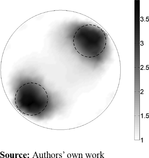
Exemplary reconstruction of two rod type inclusions using the proposed BFGS-based algorithm
Exemplary reconstruction of two rod type inclusions using the proposed BFGS-based algorithm
6. Conclusion
In this work, we presented fast numerical techniques for FE simulations in ECT. We demonstrated a fast assembly technique for the FE equation system based on an eigenvector scheme as well as Jacobian operations. The techniques are based on the linearity of the problem and take advantage of a solution by Green’s functions due to the symmetry of the FE stiffness matrix. Timing measurements showed the superior performance of the methods with respect to standard implementations. In fact, with the present approach, computations involving the Jacobian can be carried out for free, i.e. no additional effort is required as it is for known reference techniques like adjoint field methods. The techniques are applicable to other inverse problems and can also be used for different solution algorithms for inverse problems, like Kalman filters or inferential techniques. The well-structured notation of the calculations should allow researchers to easily integrate them into their own code.
The financial support provided by the Austrian Federal Ministry for Digital and Economic Affairs, the National Foundation for Research, Technology and Development and the Christian Doppler Research Association is gratefully acknowledged.
