This study aims to address the question of how generative artificial intelligence can be used to reduce the time required to set up electromagnetic simulation models. A chatbot based on a large language model (LLM) is presented, enabling the automated generation of simulation models with various functional enhancements.
A chatbot-driven workflow based on the LLM Google Gemini-2.0-Flash automatically generates and solves two-dimensional finite element eddy current models using Gmsh and GetDP. Python is used to coordinate and automate interactions between the workflow components. The study considers conductor geometries with circular cross-sections of variable position and number. In addition, users can define custom postprocessing routines and receive a concise summary of model information and simulation results. Each functional enhancement includes the corresponding architectural modifications and illustrative case studies.
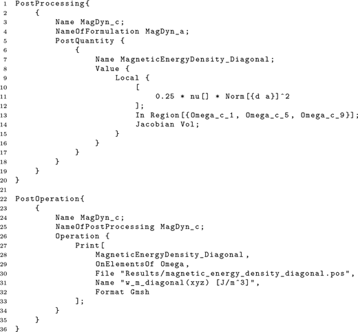
With a defined set of functionalities, the chatbot successfully sets up and solves electromagnetic simulation models. Notably, it automatically infers not only Python code but also the domain-specific language code for GetDP. The case studies conducted revealed open research challenges, particularly with regard to the question of how to ensure that results are both syntactically and semantically valid.
Currently, the application of machine learning methods to solve electromagnetic boundary value problems is an active area of research (see, e.g. physics-informed neural networks or neural operators). However, to the best of the authors’ knowledge, little research has examined the potential of artificial-intelligence-assisted generation of simulation models that prioritizes code generation and execution rather than the enhancement of numerical solution schemes. This study leverages a LLM and designs tailored workflows that contextualize it through carefully constructed system prompts.
1. Introduction
The application of machine learning (ML) methods, a subfield of artificial intelligence (AI), to the solution of electromagnetic boundary value problems (BVPs) is currently a highly active area of research. Deep neural networks for operators (Kovachki et al., 2023; Lu et al., 2021a, 2021b; Li et al., 2020) and physics-informed neural networks (Raissi and Karniadakis, 2018; Raissi et al., 2019; Karniadakis et al., 2021), in which information about the BVP (and possibly measurement data) is integrated into the loss function of the network, often aim to replace traditional numerical methods such as the finite element (FE) method. For physics-informed neural networks in electromagnetism specifically [see, e.g. Lim and Psaltis (2022); Guo et al. (2025); Rezende and Schuhmann (2025)]. Furthermore, deep neural networks have also been applied to reduced order modeling (see, e.g. He et al., 2023).
This work addresses an orthogonal problem: How can AI methods be used to reduce the time required to set up electromagnetic simulation models, rather than solving the numerical models themselves? The focus is thus on the assisted generation of simulation models, whereby the numerical scheme itself remains unaffected. A conceptually related direction has recently emerged in the computational fluid dynamics (CFD) community. In Yue et al. (2025), an AI-based multiagent framework called Foam-Agent is introduced that supports users in performing simulations based on the open source CFD software OpenFOAM (OpenFOAM Ltd, 2025). To the best of the authors’ knowledge, there are only a few works on this subject in computational electromagnetics [see, e.g. Lupoiu et al., (2025)].
Motivated by this research gap, the present work introduces a chatbot-driven workflow based on the text capabilities of the multimodal large language model (LLM) Google Gemini-2.0-Flash (Google DeepMind, 2025) that facilitates the automated generation of two-dimensional eddy current simulation models using the open source FE tools Gmsh (Geuzaine and Remacle, 2009) and GetDP (Dular et al., 1998). The study focuses on geometries consisting of conductors with circular cross-sections, whose positioning and number can be controlled by the user via natural language prompts. Further, users can define custom postprocessing routines, such as a visualization of the ohmic power loss density for a selected subset of conductors. In addition, the user is automatically provided with a textual summary of the model information and simulation results.
The remainder of this paper is organized as follows: Section 2 introduces the model problem, the main software tools and the basic workflow of the proposed chatbot prototype. Section 3 discusses architectural extensions of the workflow and case studies that demonstrate domain-specific language (DSL) code inference and automatic textual summarization. In addition, we introduce a possible encoding scheme describing what qualifies as an acceptable result from the user’s point of view. Section 4 presents an evaluation study quantifying the performance of the chatbot-driven workflow. Different LLM models are benchmarked here on exemplary problems of varying difficulty. Finally, Section 5 summarizes the main findings and outlines future research directions.
2. Overview of the basic AI workflow
This section introduces the two-dimensional eddy current model problem and briefly discusses the open source finite element tools Gmsh and GetDP, focusing on their interfacing capabilities. These tools are subsequently integrated into a chatbot-driven workflow, which is presented here in its basic form.
2.1 Model problem
As an application example, we consider the translationally symmetric eddy current problem shown in Figure 1. Since the electromagnetic fields do not change with respect to the z-direction, the problem can be treated in two spatial dimensions.
 The diagram shows a large circular domain containing multiple smaller circular regions labelled omega c 1, omega c 2, and omega c N. Each small circle represents a conductor with radius r c. A dashed line marks the distance d b n d from the boundary. The outer region is labelled omega i with sigma equals 0, and nu equals 1 over mu 0. The conductor region omega c 1 is labelled sigma C u and nu equals 1 over mu 0. The boundary is marked as a partial omega.
Sketch of the computational domain Ω: insulating domain Ωi, boundary of the domain ∂Ω and N separated conductors, each with a radius rc. The total conducting domain is . Each conductor center has at least the minimal distance dbnd to the circular boundary ∂Ω
The diagram shows a large circular domain containing multiple smaller circular regions labelled omega c 1, omega c 2, and omega c N. Each small circle represents a conductor with radius r c. A dashed line marks the distance d b n d from the boundary. The outer region is labelled omega i with sigma equals 0, and nu equals 1 over mu 0. The conductor region omega c 1 is labelled sigma C u and nu equals 1 over mu 0. The boundary is marked as a partial omega.Sketch of the computational domain Ω: insulating domain Ωi, boundary of the domain ∂Ω and N separated conductors, each with a radius rc. The total conducting domain is . Each conductor center has at least the minimal distance dbnd to the circular boundary ∂Ω
We consider separated massive conductors with circular cross-sections of radius rc and electrical conductivity σ > 0. The position of the i-th conductor is defined by its center point pi ∈ ℝ2, with i ∈ N. We denote the conducting domain as , which is surrounded by the insulating domain Ωi with σ = 0. The total domain Ω = Ωc ∪ Ωi has a circular boundary ∂Ω. Since the positions of the conductors are considered variable, it must be ensured that the boundary ∂Ω fully encloses all of them, including a minimal distance dbnd to reduce the influence of the boundary on the solution. To ensure this, the centroid of all conductors is computed, which defines the center of the circular boundary ∂Ω. The radius of the boundary ∂Ω is determined by the distance from the centroid to the outermost conductor center pi, plus the constant dbnd, see again Figure 1. We model the boundary ∂Ω as perfectly electrically conductive, i.e. σ → ∞. Furthermore, magnetic materials are excluded from this application example, so the magnetic reluctivity is ν = 1/μ0 in the entire domain.
The model is excited by imposed currents, which define the global conditions of the associated eddy current BVP: Each conductor carries a time-harmonic current of amplitude I with frequency f, respectively, angular frequency ω = 2πf. For the sake of clarity, all parameters of the model problem are summarized in Table 1.
Parameters of the eddy current model problem
| Parameter | Description | Numerical value and unit |
|---|---|---|
| rc | Radius of the conductors | 5 mm |
| dbnd | Minimum distance between the center of the outermost conductor and the boundary ∂Ω | 3rc = 15 mm |
| ν | Magnetic reluctivity | 1/μ0, with 4 π × 10–7 Vs/Am |
| σ | Electrical conductivity | 0 in Ωi, σCu = 58.1 MS/m in Ωc |
| I | Amplitude of the imposed current | 1 A |
| f = 2π/ω | Frequency of the imposed current | 50 Hz |
The physical phenomena are governed by the time-harmonic Maxwell’s equations in the magnetoquasistatic limit:
in which B is the magnetic flux density, E is the electric field, H is the magnetic field, J is the current density and is the imaginary unit. As we consider linear materials, the following constitutive laws hold:
The perfectly electrically conductive boundary ∂Ω leads to vanishing tangential components of the electric field E:
in which n is the unit external normal vector of the boundary ∂Ω.
Equations (1)–(3), together with the global conditions for the conductor currents, define an eddy current BVP that can be solved numerically using the finite element method. A commonly used finite element formulation for this type of problem is the modified A – v magnetic vector potential formulation, see, e.g. (Dular, 2023). Here, the magnetic vector potential A satisfying B = curl A is introduced in Ω, while an electric scalar potential v is defined only in Ωc. The electric field E can be expressed in terms of the scalar and vector potentials as E = –jωA – gradv. To ensure the uniqueness of the magnetic vector potential A, a gauge condition must be imposed. For the translationally symmetric model the current density J is assumed to be purely z-directed, such that the magnetic flux density B only has in-plane components, i.e. B = exBx + eyBy. This is ensured by choosing A = ezAz, which implicitly fulfils the Coulomb gauge div A = ∂Az/∂z = 0, as the component Az solely depends on the coordinates x and y.
Concisely, the A – v formulation, expressed in its weak (variational) form, can be stated follows: Seek A ∈ FA and gradv ∈ (Ωc), such that for all test functions A′ ∈ FA,0 and gradv′ ∈ 0(Ωc):
The discrete counterpart of the function space (Ω) is spanned by z-directed nodal basis functions that vanish on the boundary, i.e. Az|∂Ω = 0. The function space (Ωc) is represented by N z-directed constants, one associated with each conductor. The term denotes the voltage that can be associated to the i-th conductor. As the current Ii∈N = I is fixed for each conductor, the voltages are resulting from the finite element solution. For additional information, the reader is referred to (Dular, 2023).
2.2 Open source finite element tools Gmsh and GetDP
The computational domain Ω shown in Figure 1 is discretized using the open source finite element mesh generator Gmsh. Here, the coupling with our later chatbot-driven workflow is achieved via its Python (Python Software Foundation, 2025) application programming interface (API). This interface enables the implementation of a Python function that accepts as input a list of tuples of length 2, each specifying the coordinates of a conductor’s center pi, with i ∈ N. The number of conductors N is directly determined by the length of the input list. This procedure enables mesh generation independently of the specific number and spatial arrangement of the individual conductors. The minimal and maximal mesh characteristic sizes are defined based on the radius of the boundary ∂Ω and the radius of the conductors rc (see Table 1), to obtain a manageable number of triangles (for fast prototyping) independently of the number and spatial arrangement of the conductors. Prior to meshing, a check is performed to ensure that the conducting domains do not overlap. Furthermore, for the discretized counterparts of the conductive subdomains and the boundary ∂Ω, so-called physical groups need to be defined and stored in the resulting mesh file (“.msh” file extension), so that common material properties and boundary conditions can be assigned for the subsequent FE solver.
The A – v formulation, see equations (4), (5), is implemented in the open source finite element solver GetDP. Unlike Gmsh, GetDP cannot be interfaced directly from Python, as no dedicated API is available. Instead, solver files must be written in GetDP’s domain-specific language and stored as ASCII files with the “.pro” file extension. These solver files can then be executed via the command-line interface (CLI). After computation, the resulting field plots, e.g. for the magnetic flux density B (“.pos” file extension) can be visualized using the postprocessing facilities provided by Gmsh. It should be emphasized that the CLI commands are executed from Python through the subprocess module.
2.3 Chatbot-driven workflow
Both open source FE tools are now integrated into a chatbot-driven workflow, as illustrated in Figure 2. The chatbot is based on the free tier of Google Gemini-2.0-Flash, a multimodal LLM, but uses only its text generation capabilities. For general literature on LLMs, see (Alammar and Grootendorst, 2024). The user interface is implemented as an interactive web application using the open source framework Streamlit (Streamlit, 2025), see Figure 3. Python serves as the coordinating and automation layer, managing the interaction between workflow components.
 The diagram shows a user sending prompts through Stream lit to a system combining Python and Gemini. The prompt generates a list of coordinates labelled x y list. This connects to G m s h via Python A P I to generate a mesh file. The mesh is passed to Get D P using a file call. Get D P solves a 2 D eddy current finite element formulation and outputs visualised electromagnetic quantities such as B and J.
Sketch of the basic AI workflow
The diagram shows a user sending prompts through Stream lit to a system combining Python and Gemini. The prompt generates a list of coordinates labelled x y list. This connects to G m s h via Python A P I to generate a mesh file. The mesh is passed to Get D P using a file call. Get D P solves a 2 D eddy current finite element formulation and outputs visualised electromagnetic quantities such as B and J.Sketch of the basic AI workflow
 The interface shows a chatbot titled L L M for computational electromagnetics. Text explains the system uses Gemini 2 point 0 Flash and integrates with G m s h and Get D P. The chatbot offers to set up and solve a 2 D magnetoquasistatic boundary value problem. An example user query requests simulation with 9 conductors arranged in a square. The system indicates processing and includes references to mesh generation and electromagnetic outputs such as magnetic flux density B and current density J.
User interface of the developed chatbot: Status bar containing additional meta information (left), initial information (top) and text box for user prompts (bottom)
The interface shows a chatbot titled L L M for computational electromagnetics. Text explains the system uses Gemini 2 point 0 Flash and integrates with G m s h and Get D P. The chatbot offers to set up and solve a 2 D magnetoquasistatic boundary value problem. An example user query requests simulation with 9 conductors arranged in a square. The system indicates processing and includes references to mesh generation and electromagnetic outputs such as magnetic flux density B and current density J.User interface of the developed chatbot: Status bar containing additional meta information (left), initial information (top) and text box for user prompts (bottom)
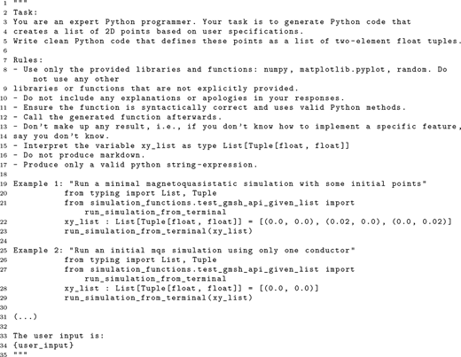
The program workflow can be summarized as follows: the user’s prompt is incorporated into a system prompt containing a task description, rules and examples (see Appendix 1.1), which is given to the LLM to generate a string of (ideally [1]) syntactically correct Python code. Then, a cleaned version of the LLM’s output string serves as the input for a function that executes the dynamically generated Python code. The Gmsh and GetDP code is static and accessed via a predefined Python wrapper function (see Section 2.2), which takes a list of coordinate tuples as input and runs the finite element simulation as a side effect. It is important to emphasize that the LLM’s weights are not updated or re-trained (that is, there is no fine-tuning); rather, the pre-trained model is contextualized at runtime via the system prompt. More precisely, the system prompt supplies task-specific instructions and context regarding the model’s input, however, it does not alter the model’s parameters. Moreover, this workflow does not employ retrieval-augmented generation (RAG) or any persistent memory mechanism: no external knowledge store is queried during generation and no state is retained beyond the immediate prompt.
3. Architectural extensions and case studies
This section presents functional enhancements to the basic AI workflow described in Section 2.3. The architectural modifications are detailed, and case studies are conducted and discussed for each autonomy level of the chatbot.
3.1 Inferring python code to generate a list of coordinate tuples
The workflow of Section 2.3 is used without further modifications to generate the exemplary results shown in Figure 4 and 5. Examples of the inferred Python code are provided in Appendix 2.1.
 The eight panels are labelled a to h. Panel a shows 12 conductors arranged in a circle of radius 0.03 metres. Panel b shows 10 conductors aligned along the y-axis. Panel c shows 100 conductors in a 10-by-10 hexagonal grid. Panel d shows conductors filling a trapezoidal slot without overlap. Panels e and f show 12 conductors placed along a sinusoidal curve between 0 and 0.2 metres. Panel g shows 5 conductors at the vertices of a square. Panel h shows 15 conductors forming the shape of the letter A.
Real parts of the current density J distributions corresponding to the models generated based on user prompts (a)–(d)
The eight panels are labelled a to h. Panel a shows 12 conductors arranged in a circle of radius 0.03 metres. Panel b shows 10 conductors aligned along the y-axis. Panel c shows 100 conductors in a 10-by-10 hexagonal grid. Panel d shows conductors filling a trapezoidal slot without overlap. Panels e and f show 12 conductors placed along a sinusoidal curve between 0 and 0.2 metres. Panel g shows 5 conductors at the vertices of a square. Panel h shows 15 conductors forming the shape of the letter A.Real parts of the current density J distributions corresponding to the models generated based on user prompts (a)–(d)
 The diagram shows a user interacting through Stream lit with a system using Python and Gemini. An extended prompt generates coordinate data and additional Get D P code files. The coordinates are passed to G m s h via Python A P I to create a mesh file. Get D P receives the mesh and additional code through command line execution. It solves a 2 D eddy current finite element formulation and outputs visualised results, highlighting selected conductors for ohmic power loss density.
Real parts of the current density J distributions corresponding to the models generated based on user prompts (e)–(h)
The diagram shows a user interacting through Stream lit with a system using Python and Gemini. An extended prompt generates coordinate data and additional Get D P code files. The coordinates are passed to G m s h via Python A P I to create a mesh file. Get D P receives the mesh and additional code through command line execution. It solves a 2 D eddy current finite element formulation and outputs visualised results, highlighting selected conductors for ohmic power loss density.Real parts of the current density J distributions corresponding to the models generated based on user prompts (e)–(h)
It can be observed that the workflow successfully infers Python code capable of generating conductor arrangements across multiple levels of complexity. The risk of conductor overlap can be significantly reduced if the user’s prompt includes the specific value of the conductor radius rc, a parameter that is not known a priori to the LLM. The simulation models shown in Figure 5, based on identical user prompts (e) and (f), illustrate the stochastic nature of the underlying LLM. Both generated geometries are correct; however, the Python code for (e) assumes α = 1, whereas the code for (f) uses α = 100. The resulting simulation model for the user prompt (g) can be interpreted as hallucination of the LLM, that is, an output inconsistent with reality. However, such hallucinations were observed only rarely in this use case; in this instance, the effect was triggered by the inconsistent user prompt, as a square obviously has only four vertices. From the standpoint of automated model validation, a notable challenge occurs when the inferred Python code is syntactically valid, yet the resulting model exhibits an incorrect geometric interpretation (see the generated model for the user prompt (h) in Figure 5).
3.2 Inferring domain-specific language code (including meaningful examples in the system prompt)
The workflow described in Section 2.3 is extended to allow the user to define custom postprocessing routines; see Figure 6. As an application example, the visualization of the ohmic power loss density pΩ is considered, which is defined as a time-averaged quantity as follows:
 The plot displays seven conductors positioned along a curve defined by y equals 20 x squared within the range negative 0.05 to 0.05 metres. Each conductor shows a colour-mapped current density labelled J x y z in ampere per metre squared real part. The arrangement forms a curved arc with varying positions along the horizontal axis.
Sketch of the extended AI workflow for dynamically generated postprocessing routines (including meaningful examples in the system prompt)
The plot displays seven conductors positioned along a curve defined by y equals 20 x squared within the range negative 0.05 to 0.05 metres. Each conductor shows a colour-mapped current density labelled J x y z in ampere per metre squared real part. The arrangement forms a curved arc with varying positions along the horizontal axis.Sketch of the extended AI workflow for dynamically generated postprocessing routines (including meaningful examples in the system prompt)
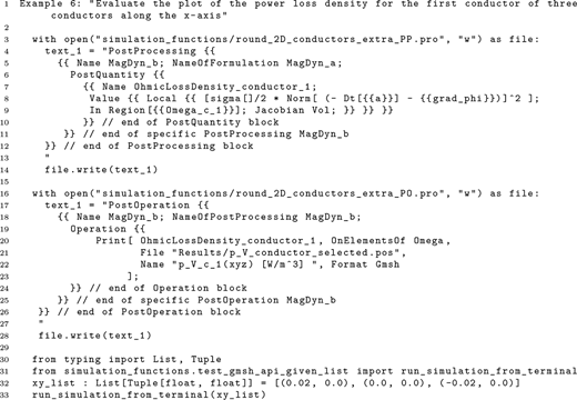
An extended system prompt is provided to the LLM, that contains GetDP code examples for a postprocessing routine, that computes and plots the ohmic power loss density pΩ only for a selected subset of conductors, see Appendix 1.2. Internally, GetDP uses PostProcessing objects to define quantities based on the primary variables of the finite element formulation – here, the vector potential A and the gradient of the electric scalar potential gradv. Their visualization and output are controlled via PostOperation objects, which specify formats such as line evaluations, surface plots or data tables. The dynamically generated GetDP code is written into dedicated “.pro” files, which are then included in the main solver file. It should be emphasized that the LLM now infers code in the domain-specific language of GetDP, a language on which, most likely, Google Gemini-2.0-Flash has been trained considerably less such that the LLM’s internal knowledge (cf. (Huyen, 2025, p. 301)) about GetDP is most likely quite low.
The extended workflow leads to the exemplary result shown in Figure 7. Further examples of the LLM outputs are provided in the Appendix 2.2. The results indicate that the basic workflow from the previous subsection can be extended with dynamically generated domain-specific language code. It was observed that including an adequate number of representative code examples significantly reduces syntax errors related to the GetDP language. In their absence, numerous syntax errors occurred, primarily due to missing or superfluous curly brackets.
 The plot shows a circular domain with multiple conductors, where only one conductor is highlighted with colour-mapped values of power loss density labelled p subscript omega in watts per metre cubed, real part. The remaining area appears uniform. The visual confirms that power loss density is computed and displayed only for the selected conductor based on the specified condition.
Left: Real part of the current density J corresponding to the simulation model resulting from user prompt (i), right: Customized postprocessing routine, see user prompt (i)
The plot shows a circular domain with multiple conductors, where only one conductor is highlighted with colour-mapped values of power loss density labelled p subscript omega in watts per metre cubed, real part. The remaining area appears uniform. The visual confirms that power loss density is computed and displayed only for the selected conductor based on the specified condition.Left: Real part of the current density J corresponding to the simulation model resulting from user prompt (i), right: Customized postprocessing routine, see user prompt (i)
3.3 Inferring domain-specific language code (excluding meaningful examples in the system prompt)
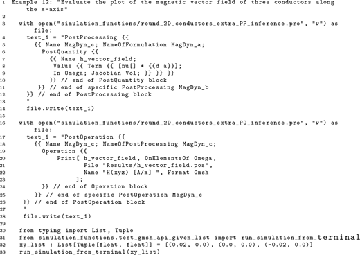
In Figure 8, the main difference to the previous architecture presented in Figure 6 is that (ideally) syntactically and semantically correct domain-specific language code is generated without having any relevant examples in the system prompt. The goal of this architectural modification is to enable valid responses to user prompts such as:
 The diagram shows a user interacting through Stream lit with a Python-based system using Gemini. An extended prompt generates coordinate data and inferred Get D P code files. The coordinates are sent to G m s h via Python A P I to generate a mesh file. Get D P receives the mesh and code through command line execution and solves a 2 D eddy current finite element formulation. The output shows magnetic energy density values plotted only at selected conductors within a circular domain.
Sketch of the AI workflow for dynamically generated postprocessing routines (excluding meaningful examples in the system prompt)
The diagram shows a user interacting through Stream lit with a Python-based system using Gemini. An extended prompt generates coordinate data and inferred Get D P code files. The coordinates are sent to G m s h via Python A P I to generate a mesh file. Get D P receives the mesh and code through command line execution and solves a 2 D eddy current finite element formulation. The output shows magnetic energy density values plotted only at selected conductors within a circular domain.Sketch of the AI workflow for dynamically generated postprocessing routines (excluding meaningful examples in the system prompt)
Using nine conductors that are positioned along a rectangle such that one point is at the center (intersection of the diagonals) and the other eight are distributed along the edges of the rectangle, evaluate the plot of the magnetic energy density in terms of the magnetic vector potential vector field within the frequency domain only for the central conductor and the conductors on the first and third bisectors of the rectangle.
An exemplary system prompt can be found in the Appendix 1.3.
The distinctive property of this kind of user prompts is that, at the same time:
these user prompts build upon examples within the system prompt discussed in previous posts such as “only for the central conductor” (cf. Section 3.2) and “along a rectangle” (cf. Section 3.1); and
these user prompts refer to examples that are not within the system prompt such as “the magnetic energy density.”
Considering the visualization of the magnetic energy density wm, recall its definition as a time-averaged quantity as follows:
A meaningful user prompt provides the LLM-based chatbot with sufficient knowledge regarding (II) such that syntactically and semantically correct DSL code can be inferred. For example, the above-mentioned user prompt has to be extended in such a way such that a contextual answer is received that conforms with the user’s expectation. More precisely, the following sentence has to be added to the above-mentioned user prompt:
Mind that the following three constraints regarding the magnetic energy density formula should be satisfied: (1) the correct factor 0.25 is present; (2) the material relation between the magnetic flux density vector field and the magnetic vector field holds to be true w.r.t. the reciprocal permeability, i.e., nu; (3) the expression is simplified by using norms.
Some observations concerning the inferring of domain-specific language code without using meaningful examples in the system prompt within the chatbot-driven workflow are:
The lack of the extension for the above-mentioned user prompt may result in:
syntactically incorrect code within the context of the DSL;
syntactically correct code that is semantically incorrect within the context of the underlying physics (e.g. using a factor of 0.5 vs. 0.25); and
syntactically correct code that behaves semantically correct within the context of the underlying physics, though, semantically incorrect within the context of the DSL (e.g. using the magnetic flux density instead of the magnetic vector potential as primary numerical solution quantity).
Given the system design at hand, there are still many optimization paths regarding the overall prompt engineering to, for example, balance the provision of knowledge by user prompts and system prompts. An interesting approach could be the use of a curated prompt store in a similar manner to a feature store [see, for example, Huyen, (2022), pp. 325ff] in other ML systems.
3.4 Inferring a textual summary of the AI workflow’s output
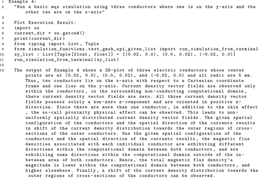
The main extension of the previous section’s workflow is the following: a function is added that executes a second LLM API-call. Its input is the output of the function that executes the first LLM API-call; and its output is a textual summary, see Figure 9. Note that there is a system prompt that contains meaningful examples and rules for structuring the output format of the textual summary, see Appendix 1.4. In other words, the dynamically generated syntactically and semantically (ideally) correct code is translated into a textual summary that expresses the physical meaning of the code in a natural language.
 The diagram shows a user providing a prompt through Stream lit requesting both a simulation and a textual summary. The system generates coordinate data and Get D P code, which are passed to G m s h to create a mesh file. Get D P solves the 2 D eddy current finite element formulation and produces visual results. In parallel, Gemini processes the output using a system prompt to generate a textual summary describing effects such as current distribution. Both numerical results and the generated explanation are presented.
Sketch of the AI workflow for dynamically generated textual summaries
The diagram shows a user providing a prompt through Stream lit requesting both a simulation and a textual summary. The system generates coordinate data and Get D P code, which are passed to G m s h to create a mesh file. Get D P solves the 2 D eddy current finite element formulation and produces visual results. In parallel, Gemini processes the output using a system prompt to generate a textual summary describing effects such as current distribution. Both numerical results and the generated explanation are presented.Sketch of the AI workflow for dynamically generated textual summaries
A couple of observations and conceptual challenges regarding the textual summary within the chatbot-driven workflow are:
Specifically, the description regarding the skin- and the proximity-effect is reasonable to a certain degree. Since a well-defined metric for quantifying potential improvements in the quality of a textual summary is currently lacking, it remains unclear whether incorporating the skin depth as an additional physical entity in the code would yield a more nuanced textual summary.
Generally, the translation of code into natural language seems to work well to a reasonable extent, see Figure 10. Due to the above-mentioned lack of a quality metric for a textual summary, though, it remains unclear whether translating numerical simulation plots (i.e. images) into text or translating numerical simulation numbers (i.e., tabular data) into text could lead to a more nuanced textual summary.
 The ten circular conductors are arranged in a ring inside a larger domain. Vector arrows indicate the field distribution over selected conductors. Two colour scales are shown. One labelled J of x y z in ampere per square metre shows values from about 1.25 e plus 4 to 1.33 e plus 4. Another labelled p V combined of x, y, and z in watts per cubic metre shows values from 0 to about 1.76. Caption states simulation with ten conductors and ohmic loss density plotted at every second conductor.
Above: Real part of the current density J and custom postprocessing routine for the ohmic power loss density pΩ generated based on user prompt (j). Below: dynamically generated textual summary of the results
Note(s): The plot shows a 2D simulation of 10 conductors arranged in a circle. The ohmic loss density, representing power dissipation due to current flow, is displayed for every second conductor (conductors 1, 3, 5, 7, and 9). The positions of the conductors’ center points are determined by a circle of radius 0.02, with coordinates calculated using sine and cosine functions, reflecting their circular arrangement. Due to the alternating current, both skin and proximity effects are present, leading to nonuniform current density distributions within the conductors and influencing the ohmic loss density. The skin effect causes current to concentrate near the surface of each conductor, while the proximity effect modifies the current distribution due to the presence of neighboring conductors
The ten circular conductors are arranged in a ring inside a larger domain. Vector arrows indicate the field distribution over selected conductors. Two colour scales are shown. One labelled J of x y z in ampere per square metre shows values from about 1.25 e plus 4 to 1.33 e plus 4. Another labelled p V combined of x, y, and z in watts per cubic metre shows values from 0 to about 1.76. Caption states simulation with ten conductors and ohmic loss density plotted at every second conductor.Above: Real part of the current density J and custom postprocessing routine for the ohmic power loss density pΩ generated based on user prompt (j). Below: dynamically generated textual summary of the results
Note(s): The plot shows a 2D simulation of 10 conductors arranged in a circle. The ohmic loss density, representing power dissipation due to current flow, is displayed for every second conductor (conductors 1, 3, 5, 7, and 9). The positions of the conductors’ center points are determined by a circle of radius 0.02, with coordinates calculated using sine and cosine functions, reflecting their circular arrangement. Due to the alternating current, both skin and proximity effects are present, leading to nonuniform current density distributions within the conductors and influencing the ohmic loss density. The skin effect causes current to concentrate near the surface of each conductor, while the proximity effect modifies the current distribution due to the presence of neighboring conductors
Notice that the conceptual challenge with regard to a quality metric for a textual summary is linked to the fundamental conceptual challenge of how to enable an automated LLM-workflow evaluation.
3.5 Aspects of semantic and syntactic sources of potential failure in the AI workflow
The workflows presented in Sections 3.1–3.4 introduce different levels of capabilities in the generated code. Here, we introduce a possible encoding scheme that describes what qualifies as an acceptable result from the user’s point of view.
Considering the workflow described in Section 3.1, the dynamically generated Python code must first satisfy the syntax and semantics of the Python programming language. Theoretically, all combinations of the truth values listed in Table 2 could occur. Syntax errors can arise, for instance, if brackets are left unclosed, as in “(a + 1”, or if reserved keywords are used as variable names. Semantic errors can occur, for example, when a variable is used before it is defined, or when operations are incompatible with the types of their inputs, as in “’a’ + 3”. While syntactic errors are detected during parsing, both syntax and semantic errors are ultimately revealed when the generated code is executed.
Boolean values representing the syntax and semantics of the dynamically generated python code
| Python syntax | Python semantics |
|---|---|
| ✗ | ✗ |
| ✗ | ✓ |
| ✓ | ✗ |
| ✓ | ✓ |
More subtle errors occur when the generated Python code is both syntactically and semantically correct, but the resulting geometry does not match the user’s expectations, consider, for example, the resulting model for the user prompt (h) in Figure 5. Consistent with the concepts of syntax and semantics, an additional layer can be introduced to capture geometric information, which gives rise to the tensorial structure depicted in Figure 11. This structure can be understood as follows: an output is considered acceptable to the user only if it is valid on both the syntax and semantic levels; applied to both the Python code and the corresponding geometry.
 The diagram shows a vertical stack of alternating red and green cubes. Arrows point from the cube structure to text labels, geometry, syntax, semantics, and Python code syntax and semantics. A symbol between them indicates interaction. The visual suggests mapping between geometric representation and programming structure.
Stack of syntaxes and semantics for workflow as in Section 3.1
The diagram shows a vertical stack of alternating red and green cubes. Arrows point from the cube structure to text labels, geometry, syntax, semantics, and Python code syntax and semantics. A symbol between them indicates interaction. The visual suggests mapping between geometric representation and programming structure.Stack of syntaxes and semantics for workflow as in Section 3.1
Conceptually, for the workflow presented in Sections 3.2 and 3.3, two additional layers are introduced (see Figure 12). Here, also the inferred GetDP code might contain syntax errors, such as improperly matched curly brackets. Semantic errors arise when a field variable is accessed that does not correspond to a primary variable in the FE formulation. Again, these errors are not difficult to detect, as GetDP’s parser will produce an error message. Again more subtle, the inferred formula for the magnetic energy density wm must be physically consistent. In this context, syntactical errors can be interpreted as operations that violate mathematical syntax, such as the addition of scalar and vector fields, consider, e.g. the expression “v + A”. Semantic errors, on the other hand, refer to operations that are mathematically valid but physically meaningless, for example, the addition of different vector field quantities such as “E + H”.
 The diagram shows stacked red and green cubes arranged diagonally. Arrows connect the cubes to labels, Python code syntax and semantics, geometry syntax and semantics, Get D P syntax and semantics, and physics syntax and semantics. Small symbols between labels indicate relationships. The layout shows layered interaction between programming, geometry, solver, and physical modelling.
Stack of syntaxes and semantics for workflow as in Section 3.2 and 3.3
The diagram shows stacked red and green cubes arranged diagonally. Arrows connect the cubes to labels, Python code syntax and semantics, geometry syntax and semantics, Get D P syntax and semantics, and physics syntax and semantics. Small symbols between labels indicate relationships. The layout shows layered interaction between programming, geometry, solver, and physical modelling.Stack of syntaxes and semantics for workflow as in Section 3.2 and 3.3
The dynamically generated textual summary (see Section 3.4) introduces yet another layer. In this context, syntactical errors can be interpreted as grammatical or spelling errors in the generated text. Semantic errors, on the other hand, occur when there is a mismatch between the actual generated model and its corresponding textual summary.
4. Evaluation of the AI workflow
The goal of this section is to provide some quantifiable results regarding the presented AI workflow that lay the foundation for more in-depth evaluation analysis in future research.
4.1 Setup
Our proposed evaluation setup is as follows:
We choose three benchmarking user prompts (see Benchmarking user prompts (basic, intermediate, advanced) for the evaluation of the AI workflow that are representing electrical conductors in different geometrical configurations (recall Section 3.1) and postprocessing routines (recall Section 3.3)). These prompts represent different levels of complexity, that is, basic, intermediate and advanced. The complexity of user prompts is assessed across the three tiers based on the ambiguity potential and the electromagnetic computation demands as judged by a subject matter expert. Mind that the system prompts (cf. Appendix 1) are kept constant for all runs:
Basic: “Run an MQS simulation with ten conductors placed along an outer circle (with a radius of 4 cm) and ten conductors placed in an inner circle. Note that each conductor has a radius of 5 mm. Ensure that the conductors are not overlapping. Plot the ohmic power loss density only for the inner circle’s conductors.”
Intermediate: “Run an MQS simulation model with a proper number of conductors that fill completely a symmetric trapezoidal slot form. Ensure that, at each vertex of the symmetric trapezoidal slot form, there is a conductor. Avoid that the conductor cross sections are overlapping when considering the radius = 0.005 m. Please enlarge the spacing between the conductors. Plot the ohmic power loss density only for the bottom row of conductors.”
Advanced: “Run an MQS simulation with a proper number of conductors that are formed like a Milliken-type conductor. Use at least 100 conductors. Arrange this number of conductors in separated segments that are kind of pie-shaped. Typically you need 6 of them. Leave some space in the inner part of the total cross-section (ca. 0.01 m) such that there is no conductor. Leave also some space between the segments such that their separation is clearly visible. Avoid that the conductor cross sections are overlapping when considering the radius = 0.005 m. Please enlarge the spacing between the conductors. Plot the ohmic power loss density only for the conductors of each segment that are along the boundary of the segment.”
Since the model Gemini-2.0-Flash is expected to be deprecated by publication (cf. Google DeepMind, 2026a), we select the following five models for the analysis:
Gemma-3-1b-It
Gemma-3-27b-It
Gemini-2.5-Flash-Lite
Gemini-2.5-Flash
Gemini-3.1-Fash-Lite
Gemma models are lightweight, open-weight models built on technology similar to that of Gemini’s full-fledged, closed-source lineup. Both model families are consumed via Google’s corresponding APIs. Note that Gemini-2.5-Flash has higher input and output token prices than Gemini-3.1-Flash-Lite, which in turn exceeds Gemini-2.5-Flash-Lite (cf. Google DeepMind, 2026b). These prices indicate as a first approximation that, for the Gemini models, Gemini-2.5-Flash is the most capable, followed by Gemini-3.1-Flash-Lite, then Gemini-2.5-Flash-Lite.
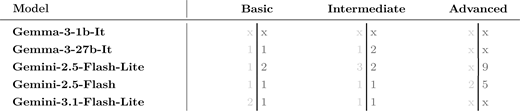
For a given model and a benchmarking user prompt, the number of tries until the first successful syntacticalAI workflow execution is counted (recall Section 3.5). Two independent attempts are conducted. If more than ten tries are needed, an “x” is marked. The results are shown in Table 3.
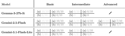
Based on the results from Table 3, it is decided to proceed with a subset of the models to analyze the successful semanticalAI workflow execution (recall Section 3.5). In Figure 13, there are reference simulation results that show one representative of the class of valid geometrical configurations and valid postprocessing routine executions associated with each benchmarking user prompt. Given these reference simulation results, a subject matter expert evaluates each successful syntacticalAI workflow execution whether there is (a) a valid geometrical configuration and (b) given (a), whether there is a valid postprocessing routine execution in the sense of that they are members of the class of valid geometrical configurations and valid postprocessing routine executions, respectively.
For example, for one attempt, if there are eight valid geometrical configurations out of ten successful syntacticalAI workflow executions, then 8 / 10 is recorded. Given the eight valid geometrical configurations, if there are five valid postprocessing routine executions, then 5/8 is recorded. In total two attempts for each pair of models and benchmarking user prompts are conducted. The results are summarized in Table 4.
For a given model (Gemma-3-1b-it, gemma-3-27b-It, Gemini-2.5-Flash-Lite, Gemini-2.5-Flash and Gemini-3.1-Flash-Lite) and a given benchmarking user prompt (basic, intermediate, advanced), the number of tries until the first successful syntacticalAI workflow execution is recorded. The light-gray numbers and gray numbers indicate results from the first attempt and the second attempt, respectively. An “x” indicates more than ten tries without success
 |
 The six panels are labelled a to f. The top row shows conductor arrangements labelled geometry basic, intermediate, and advanced, with increasing number and density of circular conductors. The bottom row shows corresponding power patterns labelled P P basic, intermediate, and advanced inside a circular domain. Basic shows a ring of conductors, intermediate shows a row, and advanced shows dense radial distribution. Colour scales indicate current density and power density values.
Reference simulations based on benchmarking user prompts (see Benchmarking user prompts (basic, intermediate, advanced) for the evaluation of the AI workflow that are representing electrical conductors in different geometrical configurations (recall Section 3.1) and postprocessing routines (recall Section 3.3)); “PP” denotes postprocessing
The six panels are labelled a to f. The top row shows conductor arrangements labelled geometry basic, intermediate, and advanced, with increasing number and density of circular conductors. The bottom row shows corresponding power patterns labelled P P basic, intermediate, and advanced inside a circular domain. Basic shows a ring of conductors, intermediate shows a row, and advanced shows dense radial distribution. Colour scales indicate current density and power density values.Reference simulations based on benchmarking user prompts (see Benchmarking user prompts (basic, intermediate, advanced) for the evaluation of the AI workflow that are representing electrical conductors in different geometrical configurations (recall Section 3.1) and postprocessing routines (recall Section 3.3)); “PP” denotes postprocessing
For a given model (Gemma-3-27b-It, Gemini-2.5-Flash and Gemini-3.1-Flash-Lite) and a given benchmarking user prompt (basic, intermediate, advanced) and given ten successful syntacticalAI workflow executions, the relative number of (a) valid geometrical configurations and (b) given (a), there is a valid postprocessing routine execution. The light-gray numbers and gray numbers indicate results from the first attempt and the second attempt, respectively
 |
4.2 Observations in terms of quality
Given the results in Table 3, using Gemma-3-1b-It, one is not able to receive a successful syntacticalAI workflow execution for any of the benchmarking user prompts. The advanced benchmarking user prompt seems to be the most challenging for all five models, though, Gemini-2.5-Flash appears to be the only reliable one that, on average, needs 3.5 tries for getting a successful syntactical AI workflow execution for the advanced case. The basic and the intermediate benchmarking user prompt are feasible for most of the models. However, Gemini-2.5-Flash-Lite needs, on average, slightly more tries than the other models. Given these results, we conclude that, in terms of gain of knowledge for the next evaluation step, i.e. the successful semanticalAI workflow execution analysis, it is sufficient to consider solely the models Gemini-2.5-Flash, Gemini-3.1-Flash-Lite and Gemma-3-27b-It.
Given the results in Table 4, it is clear that Gemma-3-27b-It is not able to properly lead to successful semanticalAI workflow executions for the intermediate benchmarking user prompt, more precisely, there has not been observed one valid geometrical configurations, that is, a symmetric trapezoidal slot form. In the case of the basic benchmarking user prompt, there has not been observed one valid postprocessing routine execution (given a valid geometric configuration), more precisely, the ohmic power loss density has not been plotted for the inner circle’s conductors, cf. Figure 14.
 The left side shows a circular domain with multiple conductors and vector arrows indicating field distribution. Below are colour scales for current density and power density. The right side shows stacked cubes connected by arrows to labels post processing geometry syntax and semantics, Get D P syntax and semantics, geometry syntax and semantics, and Python code syntax and semantics, indicating workflow relationships.
Left: systems result for the basic benchmarking prompt using the LLM Gemma-3-27b-It. The correct conductor arrangement was achieved, however the ohmic power loss density is wrongly plotted for the outer layer of conductors. Right: corresponding interpretation of the stack of syntaxes and semantics, cf. discussion in Section 3.5
The left side shows a circular domain with multiple conductors and vector arrows indicating field distribution. Below are colour scales for current density and power density. The right side shows stacked cubes connected by arrows to labels post processing geometry syntax and semantics, Get D P syntax and semantics, geometry syntax and semantics, and Python code syntax and semantics, indicating workflow relationships.Left: systems result for the basic benchmarking prompt using the LLM Gemma-3-27b-It. The correct conductor arrangement was achieved, however the ohmic power loss density is wrongly plotted for the outer layer of conductors. Right: corresponding interpretation of the stack of syntaxes and semantics, cf. discussion in Section 3.5
Using Gemini-3.1-Flash-Lite for the basic benchmarking prompt leads, on average, almost surely to a valid geometric configuration and, given those valid geometric configurations, on average, in 80% of cases, it leads to a valid postprocessing routine execution. Using it for the intermediate benchmarking prompt leads, on average, only in 15% of cases to a valid geometric configuration and, given those valid geometric configurations, on average, in 75% of cases, it leads to a valid postprocessing routine execution.
Using Gemini-2.5-Flash for the basic benchmarking prompt leads, on average, almost surely to a valid geometric configuration and, given those valid geometric configurations, on average, almost surely, it leads to a valid postprocessing routine execution as well. Using it for the intermediate benchmarking prompt leads, on average, only in 45% of cases to a valid geometric configuration and, given those valid geometric configurations, on average, almost surely, it leads to a valid postprocessing routine execution. Finally, using Gemini-2.5-Flash for the advanced benchmarking prompt leads, on average, in 75% of cases to a valid geometric configuration and, given those valid geometric configurations, on average, almost surely, it leads to a valid postprocessing routine execution.
Given the above-mentioned observations, it is reasonable to assume that using Gemini-2.5-Flash from Google’s AI model families will lead to successful syntactical and semanticalAI workflow executions.
4.3 Observations in terms of costs and time
Costs. The previous Section 4.2 focused primarily on the quality of the AI workflow. Regarding costs, each benchmarking user prompt (plus constant system prompt; cf. Section 4.1) averages approximately 10,000 input and output tokens such that all runs in Tables 3 and 4 total roughly €1.
Time. A single run from the Table 3 and the Table 4 takes just a few seconds. Note the up-front setup investment and ongoing maintenance, but post-setup, time-to-experimentation drops by orders of magnitude. Section 4.2 confirms acceptable results across complexity levels in seconds.
Contrast this with simulation engineers without AI tools: for the basic prompt (see Table 3), an entry-level engineer might need 8 h, mid-level 4 h and master-level 2 h to start experimenting. Subsequently, for the intermediate prompt, these times halve; and for the advanced one, the times (most likely) increase again – even for master-level simulation engineers. Even with AI tools, our proposed AI workflow likely offers lower time-to-experimentation, reliably and cost-efficiently, across more use cases.
5. Conclusion and outlook
5.1 Conclusion
This work has investigated an LLM-based chatbot for electromagnetic simulations as a minimum viable setup within the context of AI-assisted code generations and executions for numerical experiments.
More precisely, we have presented a workflow that is composed by open source FE tools (Gmsh and GetDP) and a LLM (Google Gemini-2.0-Flash) embedded within a common Python-based interface (cf. Section 2). The basic AI workflow presented in Section 3.1 infers Python code to generate a list of coordinate tuples. However, architectural extensions also enabled the inference of domain-specific language code, with and without meaningful examples in the system prompt (see Sections 3.2 and 3.3), and the inference of a textual summary of the AI workflow’s output (see Section 3.4). Finally, we have examined the semantic and syntactic sources of potential failure within the AI workflow (see Section 3.5) and quantified these by introducing an evaluation methodology in Section 4.
One key insight is that the provided setup can already enable a useful level of automation of a numerical simulation workflow which can significantly reduce the time required to generate a well-posed numerical simulation model. Mind that this time-to-experimentation is a critical metric and lowering it facilitates the accelerated exploration of, for instance, various physical scenarios and corresponding numerical simulation model configurations.
Another key insight is that relying merely on the internal knowledge of an LLM (that is, its training data) as a memory mechanism leads to insufficient outcomes of the AI workflow based on human evaluation. For example, physically relevant factors are not taken into account properly. However, by additionally using the LLM’s context (via the user prompt and the system prompt) as a further memory mechanism satisfactory outcomes of the AI workflow can be achieved.
A third key insight is that the systematic consideration of both the semantic and syntactic aspects of an AI workflow’s essential elements can offer a valuable conceptual guidance for analyzing potential failure modes. The proposed visual representation of a stack of syntaxes and semantics for the workflow’s essential elements illustrates the many combinations in which the workflow can fail. Note that this proposed visual representation is highly scalable with respect to the increasing complexity of the underlying setup, thus offering a way to conceptually manage the increased complexity.
A fourth key insight is that the shown AI workflow facilitates a declarative development style where the focus is on describing what the desired outcome is, rather than explicitly specifying how to achieve the outcome step-by-step. In many scenarios, the desired outcome is a correct numerical solution, regardless of the exact method used to achieve it. However, for validating the solution’s correctness, domain knowledge is needed – which leads to the last key insight.
The final key insight is that, due to the probabilistic nature of an LLM, it is unclear how to construct a reliable automated evaluation method for the AI workflow. The evaluation of the discussed AI workflow’s outcomes relied on human evaluation. Human evaluation defines one end of the spectrum of evaluation methods, formal verification defines the other end of the spectrum. Since most likely no formal guarantees regarding the AI workflow’s outcomes can be given, it seems at least conceivable to design semi-automated evaluation methods where human evaluation is potentially reduced to a minimum. An in-depth analysis of these ideas is left for future investigations.
5.2 Outlook
Future research and development efforts can build on the presented results in several directions. One of the most challenging and crucial efforts is the investigation of reliable (semi-) automated evaluation methods for the AI workflow. For evaluating the quality of textual summaries, for instance, one promising approach could be the usage of an additional LLM that is adapted for evaluation purposes. Another promising approach involves the use of embeddings, or vector representations (Weller et al., 2025), along with similarity metrics that enable a textual summary to be quantitatively compared to human-curated or AI-generated benchmarks.
Addressing (semi-)automated evaluation methods is also important for systematically examining the space spanned by system prompts and LLMs to find the optimal configuration for the given AI workflow.
Furthermore, examining (semi-) automated evaluation methods is also critical in the investigation of more complex AI workflows. Notice that, from a control-flow graph point of view, the discussed AI workflow can be mathematically represented as a directed acyclic graph. However, more intricate graphs are conceivable that include both sequential and parallel paths as well as iterations and selections. Moreover, if more tools (i.e. if more callable functions) are available and the planning (i.e. the construction of a control-flow graph) to complete a user-defined task is undertaken by an LLM, then the resulting system is more appropriately characterized as an AI agent rather than a predefined AI workflow. It should be noted that the research field of AI agents currently lacks a well-defined theoretical foundation (see, e.g. Huyen, 2025, pp. 276). Therefore, there are many open research questions on AI agents in the context of electromagnetic simulations that deserve a thorough investigation.
Another potential architectural extension to further enhance the developed chatbot’s functionalities is the use of retrieval-augmented generation (RAG) techniques (see, e.g. Huyen, 2025, pp. 253–275). These techniques would enable the underlying LLM to access and integrate information that the model was not, or only partially, trained on. In addition, this information is more relevant to a given user prompt than a predefined and user-prompt-agnostic system prompt. In particular, with the FE software tools (Gmsh and GetDP) integrated in the chatbot, it would be beneficial to provide to the LLM only those portions of code repositories or manuals of the FE software tools that are most relevant to a user prompt.
Finally, a valuable opportunity for future work involves expanding the set of open source numerical tools beyond Gmsh and GetDP to include additional frameworks such as openCFS (Schoder and Roppert, 2025) and DeepXDE (Lu et al., 2021a, 2021b). Such an extension would enable a unified platform of diverse numerical simulation software that can be accessed by user prompts in natural language.
Note
Mind that the LLM is a probabilistic model where, even though, input and output guardrails are used, there is no complete guarantee that the expected correct structured output is generated and that this output is fully reproducible in a deterministic sense. Thus, even when given the same input, a degree of uncertainty regarding the resulting output remains.
References
Appendix 1. A system prompts
This appendix includes representative code examples from the system prompts of the workflows discussed in Section 3. Each code snippet is part of a Python multiline string that is passed to the LLM. Mind that the full system prompt that is containing a task description, some rules and examples as well as the user input placeholder is only provided for the first system prompt 1.1. For the other system prompts, only some examples are shown and, for the sake of brevity, the rest is omitted.
Note that in the system prompts, curly braces “{” and “}” serve a special function, as they are used to denote placeholders for dynamic content. Therefore, when literal braces are required in the string (i.e. not as placeholders), they must be escaped by doubling them – written as “{{” and “}}”. This ensures that the braces are interpreted as characters rather than as variable placeholders during template rendering. This is particularly necessary for the GetDP syntax code.
1.1 System prompt for inferring python code to generate a list of coordinate tuples
1.2 System prompt for inferring domain-specific language code (including meaningful examples in the system prompt)
1.3 System prompt for inferring domain-specific language code (excluding meaningful examples in the system prompt)
1.4 System prompt for inferring a textual summary of the LLM’s output
Appendix 2. LLM outputs
This appendix includes representative code examples generated by the LLM. Note that the LLM’s output is originally a multiline string. Here, we show its cleaned version, that is, the version that is actually executed by Python (2.1) and GetDP (2.2 and 2.3).
2.1 LLM outputs for inferred python code to generate a list of coordinate tuples
The Python code below generates the conductor arrangement shown in Figure 4 (as a consequence of user prompt (c)).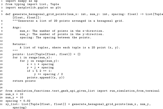
2.2 LLM outputs for inferred domain-specific language code (including meaningful examples in the system prompt)
The GetDP code below generates the custom postprocessing routine for the ohmic power loss density pΩ shown in Figure 7 (as a consequence of user prompt (i)).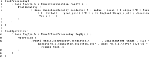
2.3 LLM outputs for inferred domain-specific language code (excluding meaningful examples in the system prompt)
The GetDP code below generates the custom postprocessing routine for the magnetic energy density wm shown on the right hand side of Figure 8 (as a consequence of the user prompt mentioned in Section 3.3).