Cooperative path following and collision avoidance of multiple robots

In recent years, the deployment of multiple robots in various domains, ranging from industrial automation to search and rescue operations, has become increasingly prevalent. This trend is driven by the ability of multi-robot systems (MRS) to improve efficiency, operational flexibility, and system robustness in accomplishing complex tasks (Drew, 2021). Cooperative path following and collision avoidance are fundamental aspects of MRS, garnering significant attention due to their critical role in enabling coordinated motion and task execution in dynamic environments (Lin and Huang, 2021). Cooperative path following entails the motion control of multiple robots while respecting inter-agent constraints and task objectives (Xiang et al., 2009). It is vital for seamless collaboration, ensuring efficient navigation and optimal resource utilization (Ni et al., 2024; Tsiu and Markus, 2020; Gan et al., 2012). This process also involves maintaining desired formations and tracking prescribed trajectories, which facilitates synchronized movement and collective behavior (Ali et al., 2005; Yu et al., 2014). However, achieving efficient cooperative path following presents significant challenges due to the inherent complexities of MRS, such as system nonlinearity, dynamic behaviors, uncertainty, and communication constraints (Raibail et al., 2022). These challenges call for advanced algorithms capable of coordinating multiple agents in real-time while adapting to environmental changes and task requirements (Verma and Ranga, 2021; Chen et al., 2024). In this work, we address the problem of path following and formation control in environments where paths and accessible regions are nonlinear and irregular. Due to these irregularities, inter-robot interactions are uncertain. Our method enables each robot to consider its position within the formation and activate collision avoidance based on the shortest inter-robot distances and predicted collision times. It is a rule-based strategy and prioritizes real-time performance.

Efficient cooperative path following is essential for enabling multi-robot systems to navigate complex environments autonomously and effectively while achieving predefined objectives. Coordinated trajectory planning among multiple robots improves energy efficiency, minimizes collision probability, and enhances system throughput (Zhou et al., 2023). Real-time cooperative swarming enables robots in MRS to dynamically reconfigure their trajectories in response to environmental perturbations and evolving task parameters, thereby enhancing system adaptability and robustness (Pike et al., 2010). This adaptability is particularly crucial in applications such as disaster response, where environmental conditions are unpredictable and rapidly changing. Furthermore, the integration of machine learning and artificial intelligence techniques has opened new avenues for enhancing the autonomy and adaptability of MRS in path-following tasks with collision avoidance. Deep reinforcement learning algorithms have demonstrated strong capability in optimizing complex motion control policies through trial-and-error interaction with simulated or real environments (Han et al., 2023; Liu et al., 2021). By learning from experience and optimizing performance over time, these algorithms can facilitate autonomous adaptation to changing environmental conditions and task requirements (Tammewar et al., 2023). Swarm robotics facilitates cooperative path following by coordinating large populations of resource-constrained robots to execute distributed tasks such as area coverage, exploration, and formation control (Zhang and Yang, 2022; Xu et al., 2024). By mimicking collective behaviors observed in natural systems such as insect swarms and animal herds, swarm robotics offers scalable and robust solutions for cooperative motion control in MRS (Eshaghi et al., 2023; Pires et al., 2021; Dias et al., 2021). Furthermore, the integration of bio-inspired principles and algorithms, such as ant colony optimization and particle swarm optimization, has proven effective in addressing challenges related to exploration and coordination in dynamic and uncertain environments (Lankford and Grimes, 2024; Gad, 2022). In this paper, we develop a control and collision avoidance framework based on inter-robot distance, time-to-collision, proximity to workspace boundaries, and desired formation positioning, allowing robots to operate within cluttered environments, accommodate non-convex body geometries, and manage nonlinear dynamics. Instead of resource-intensive trial-and-error processes, the method is rule-based and robust against complex admissible spaces.

Researchers have developed innovative system architectures for cooperative path planning and following by integrating principles from robotics, optimization, and control theory (Abdulsaheb and Kadhim, 2023; Talaei Khoei et al., 2023; Sánchez-Ibáñez et al., 2021). Centralized approaches, which involve a single centralized planner coordinating the motion of all robots, have traditionally been employed in MRS (Gulzar et al., 2018). Although centralized approaches provide globally optimal solutions, they are limited in scalability and susceptible to single points of failure. Decentralized approaches, on the other hand, distribute decision-making among robots, promoting scalability, fault tolerance, and adaptability (Tarapore et al., 2017; Chandran and Vipin, 2024). Consensus-based algorithms and decentralized control frameworks have emerged as effective methodologies for cooperative path following in MRS (Jain et al., 2018; Seidel et al., 2024; Yao et al., 2024). Through local interactions and distributed decision-making, these approaches enhance scalability and resilience, facilitating robust coordination in dynamic and uncertain environments (Bucchiarone et al., 2017; An et al., 2024; Ghassemi et al., 2019). In Na et al. (2022), pheromone-based mechanisms were utilized for inter-agent learning and communication. In contrast, this study employs deterministic control logic incorporating geometric formation constraints and predefined priority rules. Whereas the smooth vector field guidance and disturbance rejection techniques were applied in González-Sierra et al. (2023), we introduce an event-triggered switching mechanism integrated with a modular hybrid control framework. An AI-driven control architecture was designed in Sui et al. (2020) for scenario generalization, whereas our approach emphasizes rule-based strategies that ensure computational efficiency and reliable performance in structured operational contexts. This study employs time-to-collision metrics to adaptively regulate the frequency of control output updates. All robots maintain equivalent roles within the formation and make decisions autonomously, reinforcing the decentralized nature of the system. This architecture enables the robots to effectively manage nonlinear dynamics and operate under environmental uncertainty.

In this context, this study aims to design a path-following, formation-control and collision-avoidance paradigm to enable collective movements in confined space for multiple robots. We consider the system to be decentralized and robots to be cooperative. The novelty of this paper includes the following:

1. Integrate inter-robot distance, robot-boundary proximity, time-to-collision, and formation constraints into a mode-switching mechanism that governs transitions between collision avoidance, formation control, and path following. Such a framework will enable robots to handle nonconvex robot shapes and environments.

2. Employ time-to-collision metrics to trigger control updates, thereby reducing algorithmic conservativeness and improving operational efficiency. The proposed criteria are intuitive and deal with collisions directly.

3. Adapt robot trajectories based on accessible workspace and environmental boundaries, enabling dynamic adjustment of inter-robot distances for collision avoidance.

4. Select control actions from a predefined finite set, simplifying control design, reducing computational overhead, and enhancing system robustness.

In the rest of this paper, we first present the problem description, the mathematical equations, and the preliminary assumptions of the proposed research. Then, we propose the methods for target chasing and path following with algorithm design and case study. Based on the target-to-path projection, we introduce the formation control design and provide theoretical proof for stability. Furthermore, we devise the collision avoidance strategy based on inter-robot distance and collision time. The proposed algorithms are validated by simulation examples. The paper concludes with a discussion of the limitations of this study. See Table 1 for a list of symbols in this paper.

This paper considers a swarm of robots navigating along predefined paths. The robots operate within bounded environments defined by static boundary constraints. The objective is to ensure that robots follow their paths while avoiding both inter-robot and robot-boundary collisions. Each robot is modeled with an arbitrary convex polygonal shape, while environmental boundaries are defined by discrete point sequences. A collision is defined as the intersection of robot shapes or between a robot and the environmental boundary. The same holds for robot-boundary collisions. The environment contains both wide-open regions and spatially constrained (narrow) areas. Robots dynamically adjust their trajectories to navigate through narrow passages while maintaining close adherence to their original paths in wider regions. The control objective is to minimize path deviation while enabling cooperative behavior to mitigate collision risks.

We use x_i(t) ∈ R^1×2 to denote the position of Robot i at instant t in 2-dimensional Euler space. The robot moves along direction e_i(t) ∈ R^1×2, ‖e_i(t)‖ = 1, at instant t, and it can turn left/right by rotating e_i(t) in counter-clockwise/clockwise directions. Suppose that the translational and rotational speeds are ν_i(t) and ω_i(t). We use the Equation (1) to update the locations of robots.

Note that $ei⊥(t)$ is a vector perpendicular to e_i(t), and it could be either left or right to the forward direction of movement. If ω_i(t) > 0, then Robot i is turning along direction $ei⊥(t)$⁠; if ω_i(t) < 0, then Robot i is turning away from the direction $ei⊥(t)$⁠.

The path s_i = {p₁, p₂, … } of Robot i is defined by a number of points in space; p ∈ s_i is a waypoint on path s_i. The forward direction is p₁ → p₂ → …, and the backward direction is the reverse. For robot i and all the points on its path, we can find a point that is closest to the robot. Furthermore, we can find a point on the path that is d away in the forward (d > 0) or backward (d < 0) direction along the path. Vice versa, given two points p and q on the path, we can determine the distance d from which q is away from p along the path.

Conventional formation control defines the spatial configuration of robots based on their relative displacements. In contrast, this study defines robot formation based on their positions along predefined paths. Given a path, the distance between any two positions on it can be computed. Robot positions along a reference path are computed, and Robot 1 is selected as the base node. The formation is then represented by a set L = {l₂, l₃, … }, where l_i is the distance from Robot i to the base node along the path. Although the robots follow distinct paths, they move collectively while maintaining the prescribed formation. To maintain consistency in formation navigation, a common reference path is used to compute inter-robot distances, regardless of their individual trajectories.

In this paper, we consider that robots follow arbitrary known paths as a swarm. As they are not given any fixed or mobile targets to chase, we use a point on the path (or projection to the path) as such targets. We use q(t) ∈ s to denote that point q(t) is on path s at instant t. We find point $qi(t),qi*(t)∈s$ that satisfies the condition (3) below.

Note that $l¯i(t)$ is a scalar, representing that the distance from q_i(t) to $qi*(t)$ along path s_i is $l¯i(t)$⁠. We denote the energy function by (4).

We then have

In this paper, we select translational and rotational speeds from a finite set. That is,

Assume that τ₁ + τ₂ + … = 0.1 and we find $νi*(t+τ1),νi*(t+τ2),…,ωi*(t+τ1),ωi*(t+τ2),…$ by (5).

Note that under the control with (5), robots follow the targets closely, which are on their paths. Translational and rotational speeds are selected from two finite sets. Different speed combinations lead to different distances to their targets at certain times. The control outputs are those that minimize the distance to their targets.

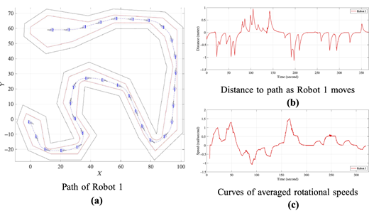
We use Robot 1 as an example (see Figure 1a). We assume that ν₁(t) ∈ {−1, 0, 1, } and

Such speeds are also used for robots in the following sections. We observe that Robot 1 can follow its path closely. The deviation from the path is given in Figure 1b. It can be seen there are large deviations whenever there are sharp turns. Robot 1 alternates among different rotational speeds, and we calculate averaged speeds in Figure 1c. We observe that the curve is above the zero line if Robot 1 turns left; the curve is below zero if Robot turns right.

In this section, we propose a formation control strategy designed to maintain relative distances between robots, enabling them to move cohesively along their respective paths. The approach involves projecting each robot’s position onto its path to compute the desired formation positions and associated tracking errors. Based on these errors, robots adjust their translational speeds to preserve the specified relative distances with respect to neighboring robots.

We use a reference path s* amid the paths of all robots to design the formation controller. Assume that Robot i is projected to point q_i on the path; l_ij is the distance from q_i to q_j. We introduce $lˆi$ to represent the distance from Robot i to the average location on the path of all the robots. We use (7) to calculate the translational speeds of all the robots. Here, we say $lˆi(t)−lˆi(t0)$ is the formation error with Robot i at instant t.

where α is a constant scalar and ν₀ is the steady state speed; N_i is a set of local robots for Robot i; if j ∈ N_i, then i ∈ N_j. The robots interact with each other locally, and the system is essentially distributed and decentralized. Note that we assume ν₀ = 1 in simulations in this paper. As long as α > 0, robots will speed up or down whenever necessary to keep the robots in a cluster. The larger α is, the faster robots falling behind will move to catch up, and the more robots in the lead will slow down.

Robots follow their paths by chasing targets on them. There will be deviations, but they are bounded and normally converge, which can be seen in Figure 1b. For simplicity, formation control can be regarded as robots moving along their paths at translational speeds by (8).

Then, we have

We denote the formation energy function by (9).

Then, we have

We observe that

Therefore, we have

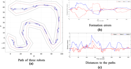
By (10), the formation errors are expected to converge over time. However, in practice, robots may not follow their designated paths precisely, especially when encountering sharp turns. Such deviations can lead to temporary spikes in formation errors, particularly during frequent directional changes. To evaluate the proposed method, we conduct a simulation with three robots, using $α=18$⁠. The assigned paths are illustrated in Figure 2a. Snapshots of the robot trajectories are captured every 21 s, demonstrating that the robots progress collectively as a cohesive group. The evolution of formation errors is shown in Figure 2b, and the corresponding distances to the paths are presented in Figure 2c. The results indicate that formation errors increase at sharp path curvatures but ultimately converge to zero by the end of the simulation.

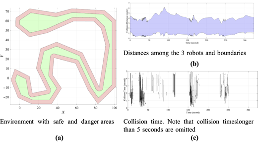
Robots are required to avoid collisions with other robots and the environment boundaries. In previous sections, we proposed algorithms that allow robots to follow designated targets and navigate along predefined paths. This section introduces methods to ensure collision avoidance with environmental boundaries and between robots. Safe Boundaries. To prevent collisions with the environment, robots must maintain a safe distance from boundary contours. We partition the accessible space into two regions: the safe area, where any point is at least a distance L from the environment boundaries, and the danger area, where any point lies within a distance L of the boundaries. For instance, in Figure 3a, the safe region is shown in green and the danger region in red. Additionally, the environment contains both narrow and wide corridors, which influence the spatial constraints of robot movement.

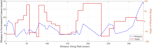
We illustrate the concept using the reference path of Robot 1, as shown in Figure 4. Suppose a robot is traversing this path. At each point along the path, we compute the shortest distances to the environment boundaries and the direction of travel, as depicted in Figure 4. The accessible corridor width along this path varies between 5.3 meters and 13.4 meters. This implies that, at minimum width, two robots can pass side by side, while at maximum width, up to four robots can traverse the corridor in parallel.

Robots are required to follow their designated paths while avoiding collisions with environmental boundaries. However, these paths may occasionally intersect with danger areas or even intrude into restricted zones near the boundaries. To ensure collision avoidance, we replace the target point defined by Equation (3) with the nearest point located within the safe area.

Collision Priority. In this paper, we consider the robots to move collectively along their paths within the accessible environment. It is assumed that the robots further along the paths have a higher priority than those behind them. This means that, given Robots i and j, if l_ij > 0, then Robot j has higher priority and does not need to consider Robot i for collision avoidance; if l_ij < 0, then Robot j has lower priority and need to consider Robot i for collision avoidance. Regardless of priority, all robots must consider environment boundaries for collision avoidance when operating within danger zones. Based on this priority scheme, collision avoidance responsibilities are primarily assigned to robots with lower priority, effectively localizing the computational burden. In our simulations, robots consider others for collision avoidance if they are located ahead along the reference path but within a 10-m range.

Shortest Distance and Collision Time for Collision Avoidance. Robots need to consider the shortest distance to other robots and the time of collision for collision avoidance. Assume that between Robots i and j, the shortest distance is d_ij(t) and the collision time is ξ_ij(t) at instant t, defined by (11). We use κ_i(t) = {κ_i,1(t), κ_i,2(t), … }, κ_i,k(t) ∈ R^1×2 to represent the shape of Robot i.

where at instant t, κ′ ∈ κ_i(t) is a point on the shape contour of Robot i and κ″ ∈ κ_j(t) is a point on the shape contour of Robot j. Note that we use (11) to obtain the shortest distance and collision time in real time. They can be used to design trigger conditions to either move forward along the paths or take collision avoidance actions. Based on shortest distances and collision times, we use (12) and (13) for collision avoidance. Moreover, calculating the shortest inter-robot distance and collision time requires computation resources. Assume that robot i updates its control by (5) and (7) at instant t and update again at t + τ_i(t). We use (14) to calculate the update interval τ_i(t).

where 0 < β < 1 is a constant.

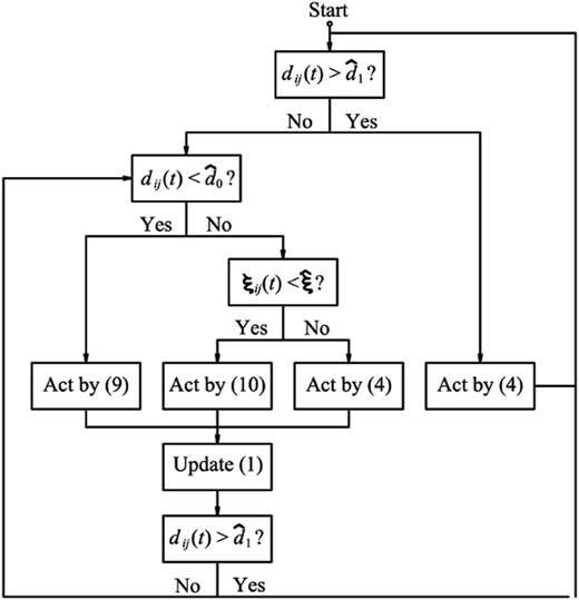
We use the flow chart in Figure 5 to denote the path following and collision avoidance strategy for the robots. Assume that robots only need to take collision avoidance actions when they are very close to collisions. As soon as they are sufficiently far apart, the robots will resume path following. Note that $ξˆ$⁠, $dˆ0$⁠, $dˆ1$⁠, $dˆ1>dˆ0$⁠, are used to trigger actions of either path following or collision avoidance.

We use Figure 2a as an example, with $ξˆ=0.5$⁠, $dˆ0=0.3$ and $dˆ1=0.6$⁠. The inter-robot distances and collision times among the 3 robots are shown in Figures 3b and 3c. The shortest inter-robot distance is 0.2875 meters and the shortest collision time is 0.102 s It can be seen that the distances and the times are uniformly positive. This means that there are no collisions.

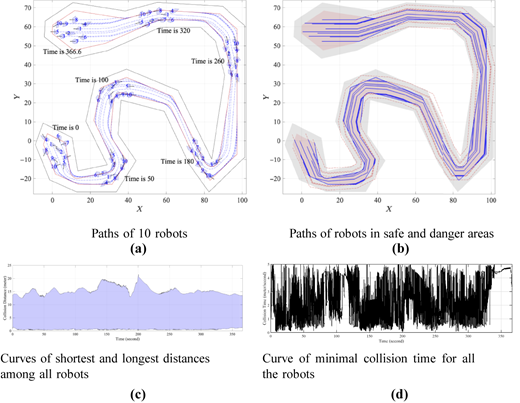
In this section, we use simulation examples to verify the performance of algorithms for path following and collision avoidance. We use 10 robots, as shown in Figure 6a. The initial directions are random, and the initial locations are in the lower left corner. The paths of robots are shown in Figure 6b with safe areas in red and danger areas in grey. The predefined paths are shown, and they are represented by blue lines inside the safe area and dashed red lines inside the danger area. The heading direction of the robots are given below.

The path of robot 1 is given below.

The distances among the robots as they move along the paths are given in Figure 6c. We observe that the distances are always positive, and 21.5 meters at most. This means that there are no collisions and any two robots are at most 22 meters apart, as the robots move as a cluster. The collision times are given in Figure 6d. The shortest time is 0.06 s. This means that robots have plenty of time for collision avoidance. The formation errors are shown in Figure 7a. We observe that the errors become nonzero whenever the robots reach the curved parts of the paths. The curved paths in Figure 6b have inner routes and outer routes, and at the same speeds, it takes robots a longer time to travel through the outer routes than the inner routes. The formation errors are bounded and eventually converge to zero. Note that for robots to focus on critical interactions, only collision events occurring within the first 5 s of each run were considered, as later events typically arise under low-density or steady-state conditions and do not reflect the core controller performance.

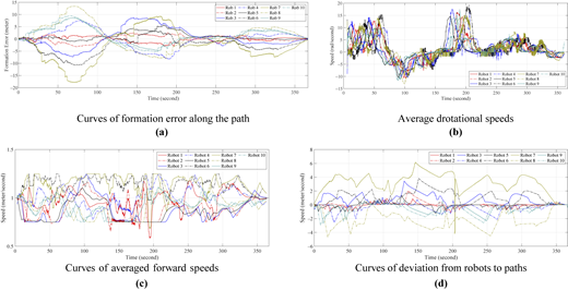
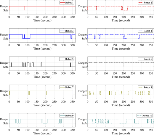
The averaged rotational and forward speeds are given in Figures 7b and 7c. The robots are turning left with averaged rotational speeds being positive and turning right with negative speeds. The robots falling behind will have translational speeds greater than 1 meter/second, and those leading will have speeds smaller than 1. Deviations from the paths of robots are given in Figure 7d. The robots move by the same controller, but their deviations are different in magnitudes and direction. The control modes of the robots are shown in Figure 8. The robots are in safe mode if they are moving along their paths by (5), they are in danger mode if they are avoiding collisions by (12) or (13). We observe that Robots 5, 8 and 10 spend more time in safe mode than danger mode, and the rest spend more time in danger mode than safe mode.

The simulation results demonstrate that the proposed control framework outperforms some state-of-the-art methods in maintaining formation and ensuring collision-free path following under constrained conditions. For instance, the minimum inter-robot distance remains strictly positive throughout the simulations, reaching a maximum of 21.5 meters, which confirms that robots maintain safe separation even in high-density scenarios. This contrasts with traditional approaches where maintaining rigid formations often leads to close-proximity risks, especially on curved paths. Additionally, the minimal predicted collision time of 0.06 s indicates that the system reacts in a timely manner to potential threats, unlike fixed-threshold systems that either overreact or miss critical collision windows. The proposed adaptive speed control allows robots on outer curves to accelerate and those on inner curves to decelerate, which mitigates the common drift or lag observed in uniform-speed models. Furthermore, the system’s mode-switching behavior highlights its ability to balance safety and efficiency. Robots transition between ”safe” and ”danger” modes based on real-time risk assessment, and the results show that Robots 5, 8, and 10 spent more time in safe mode, whereas others had to engage in frequent collision-avoidance maneuvers. This is a marked improvement over rule-based methods that treat all robots uniformly regardless of local conditions. Averaged forward speeds deviate appropriately from the baseline speed of 1 m/s—robots falling behind accelerate up to 1.3 m/s, while those in front slow to about 0.8 m/s—enabling a flexible and self-regulating cluster motion. The formation error, which spikes in curved segments due to differing path lengths, is shown to converge to zero, demonstrating the system’s robustness. Collectively, these results validate that the proposed decentralized and event-driven method offers better adaptability, communication efficiency, and formation cohesion than existing centralized or rigid schemes.

This paper presents a decentralized framework for cooperative path following and multi-robot coordination in environments with spatial constraints. By deforming predefined paths to fit accessible regions and incorporating target chasing, motion control, and formation error regulation, robots are enabled to move as a cohesive cluster while minimizing path deviation. The control logic integrates formation control, collision avoidance, and path following through event-triggered switching, with collision time used to adapt communication frequency and avoid over-communication. Simulations validate the effectiveness of the proposed approach in maintaining formation and avoiding collisions. Nonetheless, the study is subject to several limitations. The simulations are performed in idealized, static environments, which may not fully capture the uncertainties of real-world conditions. The control strategies are deterministic and may not account for stochastic disturbances or sensor noise. Additionally, the computational demands of the algorithms could hinder scalability to large robot swarms. Future research will focus on extending the framework to dynamic and uncertain environments, incorporating probabilistic modeling, and enhancing scalability through algorithmic optimization.