

The purpose of this paper is to establish and implement a direct topological reanalysis algorithm for general successive structural modifications, based on the updating matrix triangular factorization (UMTF) method for non-topological modification proposed by Song et al. [Computers and Structures, 143(2014):60-72].
In this method, topological modifications are viewed as a union of symbolic and numerical change of structural matrices. The numerical part is dealt with UMTF by directly updating the matrix triangular factors. For symbolic change, an integral structure which consists of all potential nodes/elements is introduced to avoid side effects on the efficiency during successive modifications. Necessary pre- and post processing are also developed for memory-economic matrix manipulation.
The new reanalysis algorithm is applicable to successive general structural modifications for arbitrary modification amplitudes and locations. It explicitly updates the factor matrices of the modified structure and thus guarantees the accuracy as full direct analysis while greatly enhancing the efficiency.
Examples including evolutionary structural optimization and sequential construction analysis show the capability and efficiency of the algorithm.
This innovative paper makes direct topological reanalysis be applicable for successive structural modifications in many different areas.
1. Introduction
In many engineering problems arise successive modifications of structures, as well as their computational models. Some problems only involve non-topological modifications, such as nonlinear analysis merely includes change in material properties (Bathe, 1996), while a wider range of problems involves topological modifications that change the structural layouts. For example, the topology optimization of a structure involves multi-step variation of nodes/elements on the initial design (Spillers and McBain, 2009); the sequential construction analysis (SCA) of a tall building involves solution of intermediate structures during the construction process to achieve more accurate stress or interior force distribution (Chen et al., 2006). Repetitive solutions require enormous computational effort and thus motivate the study of reanalysis methods. Reanalysis methods use the results or intermediate data generated in previous solution (generally the LDLT factor matrices) and evaluate the current structural response as accurately as possible. Comparing to non-topological problems, topological modifications bring new difficulties to reanalysis. On one hand, there is usually large change of numerical values in the resultant linear systems, and on the other hand, there are changes of size and nonzero pattern of the coefficient matrices due to node/element addition and deletion.
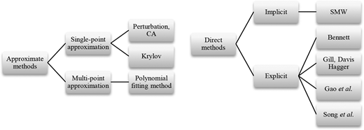
Various reanalysis methods have been proposed in last decades. As shown in Figure 1, reanalysis methods are generally classified as approximate and direct. To clarify the applicable range of reanalysis methods, relevant features of modifications are summarized. Considering the geometric scope, modifications are global or local, while considering the scale, modifications can be large or small. Additionally, modifications in some problems are single-step, while some are successive; some are located in a pre-known area, while some appear at unknown locations.
Approximate methods provide in general efficient solutions with a certain degree of accuracy loss. By assuming a set of basis vectors to approximate the modified displacement space, a reduced linear system is constructed in substitution of the original system. Selection strategies of basis vectors and solution processes for the reduced system determine the accuracy and computational complexity. According to the number of sample points in the structure variation space, single-point and multi-point approximation have been studied (Barthelemy and Haftka, 1993). An important branch of single-point approximation is derived from the perturbation series, with various research studies to improve the convergence speed (Wu et al., 2007) and accuracy (Wu et al., 2003). Based on the first few basis vectors in the Neumann series expansion, Kirsch directly reduced the initial linear system by a coordinate transformation and proposed the combined approach (CA) (Kirsch, 2009). By introducing recycled preconditioning, CA is applied to the structural topology optimization (Amir, 2015). Another branch is based on the Krylov subspace, such as the representative pre-conditioned conjugate gradient (PCG) with the factor matrices of the original structure as pre-conditioner. By building approximate functions between the structural response and modification, multi-point approximation such as the polynomial fitting method (Haftka et al., 1987) is proposed. A hybrid method combining the Fox’s polynomial fitting and CA is proposed by Zuo et al. (2012). Among approximate methods for non-topological reanalysis, several are adopted to topological reanalysis. For nodes/elements deletion, the basis vectors or the pre-conditioners are compressed by simply deleting corresponding rows and columns in the vector as well as the matrix (Wu and Li, 2005). For nodes/elements addition, Guyan reduction is widely used to reduce the stiffness matrix with added degrees of freedom (DOFs) to its original size (Xu et al., 2010). By factorizing submatrix corresponding to the added DOFs, approximate basis vectors and pre-conditioner are built for CA and PCG (Zheng et al., 2018). Combining the two-directional strategies, reanalysis method for general topological modification with nodes/elements deletion and addition happening in a single step is also proposed (Li and Wu, 2007). For structure with modified mesh, multi-grid method is introduced to deal with the inconsistency of mesh (Huang et al., 2017). Parallel CA on the multi-GPU platform is also implemented and integrated to a CAD design system (Wang et al., 2016; He et al., 2016). Approximate methods are developed into a wide range of problems including modal reanalysis (Latha and Sreenivas, 2013) and sensitivity analysis (Zuo et al., 2016). However, the approximate methods are not stable for topological modifications that greatly change the structural response. Also, as implicit methods only yield modified responses, approximate methods are not fully suitable to accumulate modifications in successive process.
Direct methods produce exact solution by implicitly updating the displacement response or explicitly updating the LDLT factor matrices. A main branch of implicit methods traces back to the Sherman–Morrison–Woodbury (SMW) solution formula (Sherman and Morrison, 1949; Woodbury, 1950) which updates displacements based on the known factor matrix of the original stiffness matrix. SMW formula lays a foundation for a series of further researches of direct methods such as the theorems of structural variation (Majid and Elliot, 1973), whose association is discussed in (Akgün et al., 2001). SMW and its variants are extremely efficient for low-rank modifications, but the efficiency will decline dramatically as rank of the modification increases, which greatly hampers their applications. In addition, a crucial obstacle of implicit methods is that only factor matrices of the original structure are accessible, so that accumulative modifications cannot be processed. Huang et al. proposed an independent coefficient (IC) method by calculating the displacements influenced by structural modifications. The method is suitable for large-scale problems with local low-rank modifications (Huang et al., 2014).
In contrast to implicit methods, explicit methods work on directly updating factor matrices before finding solutions. Bennett tried to update the modified factor matrix through SMW formula (Bennett, 1965). Gill et al. presented a set of methods to update the factor matrix when stiffness matrix is subjected to rank-one modification (Gill et al., 1972). Davis and Hagger improved this method by taking advantage of sparsity of stiffness and factor matrix and made the method suitable for large-scale problems with low-rank modifications (Davis and Hager, 2001, 2005). On this basis, Liu et al. further proposed a topological reanalysis for low-rank modifications (Liu et al., 2014a) and a reanalysis method for modification of supports (Liu et al., 2014b). In above methods, only modification in a specified form is considered and the efficiency decreases greatly as the rank of modification grows. On the other hand, by assuming that the location of modifications is pre-known and partitioning the stiffness matrix into stationary, influenced and boundary region, Gao et al. proposed an exact block-based (BB) method using block matrix inversion formula (Gao et al., 2015). As a substructure technique, it places the DOFs associated with the modified part to the end of all DOFs. However, there exists another way to perform LDLT updating. Through observation of matrix factor updating path, Law, Chan and Brandwajn proposed partial refactorization methods (Law, 1985; Chan and Brandwajn, 1986). Based on sparse solver (George and Liu, 1981) including compressed sparse row (CSR) format and graph-partition fill-ins’ reducer (Gupta, 1997), Song et al. further proposed the updating matrix triangular factorization (UMTF) and greatly enhance the efficiency for large-scale structure with local modifications (Song et al., 2014).
Workable range of direct reanalysis methods for different kinds of modifications is briefly summarized in Table I. The last column indicates the ability of each method to topological modifications with DOF addition and deletion.
Workable range of direct reanalysis methods
| Method | Distribution | Scale | Flexible location | Successive modifications | Topological modifications |
|---|---|---|---|---|---|
| SMW | Global | Very low-rank | √ | × | × |
| Bennett | Global | Very low-rank | √ | √ | × |
| Davis and Hagger | Local | Low-rank | √ | √ | √ |
| Gao et al. | Local | High-rank | × | × | √ |
| UMTF (Song et al.) | Local | High-rank | √ | √ | × |
Efficient reanalysis of topological modifications is an important subject. Among the present direct methods, only Gao’s block-based method is applied to high-rank topological modifications with limitation that all modifications happen in a pre-specified and fixed area. As UMTF shows its superiority for local high-rank non-topological modifications without any restrictions on modification locations, in this study, we focus on extending the non-topological reanalysis algorithm UMTF to deal with a series of topological modifications. The fundamental extension lies on how to deal with matrix size and nonzero pattern changes caused by topological modifications alone with some numerical value changes.
The implementation of the non-topological UMTF benefits from a fixed ordering of DOFs. An efficient implementation of the topological UMTF should require DOFs of the modified structure with added nodes/elements in a good fill-in optimized sequence and also consistent with the unmodified structure. Therefore, we introduce an integral structure including all potential elements and nodes as an essential assumption so that every structure appearing in the modification process is a substructure of the integral one with changes on nodes and elements. The current substructure is topologically modified into a target by adding/deleting certain nodes/elements of the integral structure. In sense of the global stiffness matrix of the integral structure, a modified substructure corresponds to a principal submatrix with some value changes, so that stiffness matrices of modified structures are nearly fill-in optimized. This treatment guarantees the efficiency of UMTF with versatility and robustness.
In implementation, nodes/elements addition and deletion in matrices requires expansion and shrinkage of arrays under the sparse storage format. Data arrangement is then emphasized to keep expanded or shrunk matrix in their original space, so that extra memory for topological substitutions is minimized. In the algorithm we designed, topological reanalysis is performed separately in symbolic and numerical phase. A transitional structure as an intermediate state is introduced to carry out UMTF.
An outline of this paper is as follows. In Section 2, the non-topological reanalysis method based on UMTF and fill-in reduction is briefly reviewed. In Section 3, memory setup, as well as symbolic processing for topological modification, is described in detail, and the topological reanalysis algorithm based on UMTF is explained. In Section 4, the proposed algorithm is verified and then applied to topological optimization and sequential construction analysis to show its capability and efficiency in practical problems. Section 5 is a short conclusion of the algorithm.
2. Non-topological reanalysis method
2.1 Graph partition for fill-in reduction
Direct solutions to large sparse systems of equations are based on the LDLT factorization, as shown in equation (1), where L is a unit lower triangular matrix, D is a diagonal matrix and U = DLT is an upper triangular matrix:
As the factorization proceeds, elimination of a row usually creates nonzero entries, or fill-ins, in the factor matrix L. Therefore, fill-in reduction is used to find optimized orderings of sparse matrices that can significantly reduce the number of fill-ins, as well as the associate floating-point operations.
The state-of-art technique of fill-in reduction is realized by multilevel graph partition algorithms, such as Chaco (Hendrickson and Leland, 1995) or METIS (Karypis and Kumar, 1997). Taking each DOF as a vertex and each nonzero off-diagonal as an edge connecting corresponding vertices, the algorithms treat the stiffness matrix as the adjacency matrix of a graph. The fundamental concept of the algorithms lies in the nested dissection. In each step, the graph is bisected by removing a set of vertices, named as vertex-separator S, leaving with two disjoint subgraphs L and R. An expected partition of graph requires the subgraphs are roughly equal parts and the separator is as small as possible. In the recursive nested ordering, the vertices in L is numbered first, R second and S the last. The subgraphs L and R are recursively partitioned and ordered at a number of levels by applying the same technique.
Figure 2 shows an example of a graph by two-level partition. The graph is first partitioned into subgraphs L and R by separator S. Then each subgraph is further partitioned by choosing a separator in its own domain. Finally, we obtain a fill-in reduced order by numbering the vertices in subgraphs before their separators. In the resulting matrix in equation (2), no fill-in will be generated between two different subgraphs at any level:
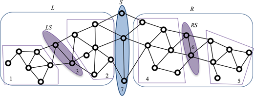
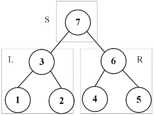
The multilevel partitioned graph can be visually represented by a tree topology, i.e. partition tree. As an example, the graph in Figure 2 leads to a partition tree shown in Figure 3. Each node in the partition tree represents a set of vertices of a subgraph or a separator. The fill-in reduced ordering of the stiffness matrix can be understood as a postorder traversal of the partition tree.
2.2 Updating matrix triangular factorization
As an explicit reanalysis method, UMTF directly updates the factor matrix L by accurately identifying the impact of structural modifications on the factor matrix and recalculating only the affected part. Non-topological structural modification implicates change of the stiffness matrix K in value. Taking a row as the smallest unit, impact of a value change in the stiffness matrix K on the factor matrix L is concluded by Rule 1:
Rule 1(Factor Change Rule): In LDLT factorization, modification of a row in the stiffness matrix K directly affects the values of this row in the factors U(LT) and D and then affects rows corresponding to the columns where nonzero entries of this row are.
As a by-product of fill-in reduction by graph partition, when a structure is modified locally, only a small subset of the entries in the factor matrix is affected. Therefore, by recalculating this part, UMTF method can greatly reduce the computation cost, while keep the precision unaffected in comparison to a full factorization. The affected part of the factor matrix caused by a change in stiffness matrix can be visually demonstrated in the partition tree as described in Rule 2:
Rule 2(Subtree Change Rule): In LDLT factorization, modification of stiffness related to a DOF only affects DOFs of the corresponding node and each parent node backtracking to the root in the partition tree, whereas the rest of the factorization results remain unchanged.
For example, in Figure 4, if the stiffness entries related to node 2 are modified, only those factor matrix entries of nodes 2, 3, and 7 are necessary to be recalculated; similarly, if the stiffness related to node 6 is modified, only entries of nodes 6 and 7 are affected. The modification path starts from this node and backtracks to the root, whereas the nodes not affected remain numerically unchanged. More details regarding sparse solutions, fill-in reduction and UMTF approach for local high-rank structural modifications can be found in (Song et al., 2014).
3. Reanalysis of topological modification
Besides mere numerical value changes in stiffness and its factor matrices, topological modification includes activation or inactivation of nonzero entries (corresponding to elements) as well as DOFs (nodes) in the matrices. This section shows how UMTF is further extended to a topological reanalysis method.
The efficiency of UMTF heavily relies on the sparsity of the factor matrix. Therefore, it is necessary to maintain a fill-in reduced ordering for the stiffness matrix of the structure with added DOF and nonzero entries brought by topological modifications. Meanwhile, as the UMTF uses the factor matrix of the original structure, the new ordering should be consistent during modifications so that UMTF is workable. To address above requirements, an ordering scheme for topological UMTF is required to guarantee the efficiency of UMTF for topological problems.
In accord with UMTF, the proposed topological reanalysis is based on the sparse solver, where the stiffness matrix and factor matrix is stored in the compressed sparse row (CSR) format. Therefore, auxiliary processing is designed for matrices expansion and shrinkage under the CSR format.
Based on the discussions above, the proposed topological reanalysis can be split into symbolic phase that handles symbolic expansion or shrinkage of the principal submatrices and numerical phase that updates matrix entries in value by UMTF.
An outline of this section is as follows. The fill-in reduced ordering scheme for structure with topological UMTF is described in Section 3.1. Detailed memory setup for topological UMTF is introduced in Section 3.2, followed by the necessary auxiliary processing for matrix storage/arrays expansion and shrinkage in Section 3.3. To the end, the program flowchart is illustrated in Section 3.4.
3.1 The integral structure and direct reanalysis algorithm
Rule 1 in UMTF reveals a general principle to update the factor matrix L and D when the stiffness matrix is subjected to arbitrary value modifications. The efficiency of UMTF is heavily dependent on the fill-in reduced ordering that limits the number of rows affected by structural modifications. This can be clearly observed by Rule 2. In the binary partition tree, modification in a subtree will not propagate to the other one. As a result, local modification requires at most not much more than half computational work of a full refactorization.
A primary challenge brought by topological modifications is to maintain a fill-in optimized pivoting sequence to stiffness matrix of the modified structure so that UMTF is workable. Adding some nodes/elements generally complicates the nonzero pattern of the stiffness matrix, and leads to invalidation of the current partition tree as well as the fill-in optimized sequence. Meanwhile, UMTF makes use of factorization of the current stiffness matrix, which implies the relative pivoting sequence of any two nodes in the current structure should not be reversed in the target structure. In other words, there should be a unified fill-in optimized sequence to satisfy these requirements.
To meet above requirements, we introduce an integral structure which includes all potential elements and nodes appear in the modification process as an initial model, and we topologically modify a structure to another by adding/deleting some nodes/elements in the frame of integral structure. During the whole modification process, structures before and after modification are all substructures of the integral structure. Correspondingly, the pivoting sequence of DOFs of any substructure is a sub-pivoting sequence of the integral one, and the corresponding stiffness matrix is a principal submatrix of the integral matrix with modifications in value, namely the modified principal submatrix. Therefore, we prevent the partition tree from invalidation, which guarantees that any stiffness matrix in the modification possesses always in a nearly fill-ins optimized pivoting sequence. The concept of the integral structure exists in a series of practical problems, such as the maximum design domain in topology optimization, the completed building in sequential construction analysis, etc.
3.2 Memory setup for topological updating matrix triangular factorization
UMTF uses the compressed sparse row scheme (CSR) for economical storage of stiffness matrix K and factor matrix L. For symmetric matrix K, only the upper triangular part is stored. CSR uses three arrays, IA(0:n), JA(nnr) and PA(nnr) to represent the matrix K. Here n denotes the order of the matrix and nnr denotes the number of non-zeros in the matrix. PA(k) records numerical value of k-th nonzero entry of the matrix in a row-oriented order and JA(k) records associated column index. The integer IA(i) is the index of the last entry of the i-th row in the PA(nnr) and JA(nnr), i.e. {(PA(k), JA(k))|IA(i-1)<k≤IA(i)} build up the i-th compressed row (George and Liu, 1981).
As an example, arrays IA, JA, PA in Table II represent the 7 × 7 symmetric global stiffness matrix in equation (3):
IA and JA reveal the sparsity pattern of the matrix and therefore are called symbolic matrix, while PA is called the value matrix. A similar data structure with arrays IU, JU and PU is established for the factor matrix U or D and LT (shortened as U/DLT). D together with LT occupies the same memory as U, as storage of the unit diagonal entry in LT can be omitted. The sizes of the value matrices PA and PU for the integral structure (for a given ordering) are constant.
To implement a topological modification from the original structure to terminal state with a known integral structure, it is necessary to reserve arrays as shown in Table III.
Fixed arrays in memory
| (IK, JK) | Symbolic stiffness matrix of the integral structure |
| (IA, JA) | Symbolic stiffness matrix of the target structure |
| (IU, JU) | Symbolic factor matrix of the current structure |
| (IV, JV) | Symbolic factor matrix of the target structure |
| PA | Numerical stiffness matrix |
| PU | Numerical factor matrix |
At the beginning of the reanalysis process, all the arrays above are allocated with memory space required by the integral structure, and always reside in the originally assigned space during the whole process. In each step, entries in array (IA, JA, PA) and (IU, JU, PU) move backward or forward. The arrays are pseudo-prolonged or truncated to meet the CSR format of the target structure, without physically change the length of the arrays.
It is noted that integer symbolic matrices (IK, JK), (IA, JA), (IU, JU) and (IV, JV) can be greatly compressed by the concept of super-equation (Chen et al., 2003). Generally, factor matrix inevitably involves a large number of fill-ins and consequently occupies several times of memory space than the stiffness matrix. As a result, value matrix PA and PU are predominant in memory requirement for the proposed algorithm, especially PU. Comparing with full analysis, extra memory space are mainly required for IA, JA of the integral structure, and IV, JV of the target structure, which is insignificant compared to PA and PU.
3.3 Symbolic phase – matrix storage manipulation
In this section, matrix storage/arrays expansion before the numerical phase and shrinkage after the numerical phase are described in detail. Regardless expansion and shrinkage, the key point to manipulate the data space movement is a map from the union (larger) DOFs to the sub-collection (smaller) DOFs:
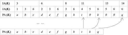
Take transformation between the smaller matrix Ks and the larger matrix Kl shown in equation (4) as example. In the shrinkage process, we start with Kl stored in IA, JA and PA, as shown in Table IV(a). The symbolic stiffness matrix of the target structure Ks can be compressed from Kl. A map MAPT of DOFs from Kl to Ks is built, as shown in Table V, here 0 indicates that the DOF is inactive in the smaller structure Ks. Then a traversal of JA is processed to map the column indexes in JA(i) to MAPT(JA(i)), where entries in the deleted row or column are assigned to 0. The number of active nonzero entries in each row are recounted and written into IA at the same time. The intermediate data in arrays are shown in Table VI. Finally, array JA as well as PA are compressed by sequentially pushing forward the active entries to the beginning of the array, and IA is rebuilt. The resultant array of Ks is again represented by IA, JA and PA in Table VII.
Stiffness matrix Kl presented in IA, JA, PA
| IA(Kl) | 3 | 6 | 8 | 11 | 13 | 14 | ||||||||
|---|---|---|---|---|---|---|---|---|---|---|---|---|---|---|
| JA(Kl) | 1 | 3 | 6 | 2 | 3 | 6 | 3 | 6 | 4 | 5 | 6 | 5 | 6 | 6 |
| PA(Kl) | a | b | c | d | e | f | g | h | i | j | k | o | p | q |
In terms of the expansion process, to avoid complete symbolic re-assembly caused by newly added entries, the symbolic matrices IA(Kl), JA(Kl) are tailored from arrays IK and JK of the integral structure by the same approach used in shrinkage. It is to note that PA(Kl) cannot be obtained by this way. The symbolic matrices of Ks in IA, JA are directly substituted by IA(Kl), JA(Kl). After that, the array PA(Ks) is prolonged to PA(Kl). The map MAPT in Table V identifies if an entry of Kl is active in the current matrix Ks. A traversal from the end to beginning of IA(Kl) and JA(Kl) is processed to stretch the PA(Ks) to the preliminary PA(Kl). To be specific, if an entry is newly added, set its value temporarily to zero. If the entry is pre-existent, extract its value from the current queue end of PA(Ks) once a time. Owing to increase of entries, index of an entry in PA of Kl will not be smaller than its index in PA of Ks during the manipulation, so that data trampling in array PA will not happen. The process and resultant array with zero entries are shown in Figure 5.
Manipulation of the symbolic factor matrix is different from the stiffness matrix. Directly constructing the symbolic factor matrix of the target substructure by a shrinkage of that of the integral structure may contain some extra fill-ins that are inactive in the target state. This will lead to an overestimation of modified rows and cause waste of computational resource. Therefore, factor matrices of target structures need an extra step of symbolic decomposition to find their symbolic part stored in array IV and JV. After that, with symbolic matrix IU, JU of current state and IV, JV of target state, the manipulation of entries in numerical factor matrix shares a similar scheme of stiffness matrix. The symbolic matrices of current and target state are checked together to determine if an entry is modified or not, which is also because of presence of extra fill-ins mentioned above.
3.4 Flowchart of topological reanalysis
In this section, a complete flowchart is given in Figure 6 based on previous discussions to accommodate successive general modifications with DOF/element addition and deletion in one single step.
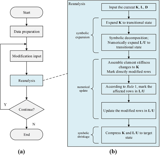
As given in Figure 6(a), the successive topological reanalysis consists of a data preparation to find the symbolic matrix for the integral structure, followed by a loop of modification input and reanalysis.
The data preparation includes: (1) input the symbolic stiffness matrix of the integral structure; (2) perform the fill-ins reduction; (3) permute the symbolic stiffness matrix; and (4) copy and save the symbolic matrix.
In reanalysis, we split the topological modification into symbolic and numerical phase, and the symbolic phase for DOF/element addition and deletion is treated individually. Nevertheless, the numerical modification caused by addition and deletion can be treated equally without discrimination. Therefore, we introduce a “transitional structure,” which is the union of the structures before and after modification and on which UMTF is implemented.
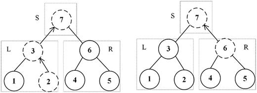
As shown in Figure 6(b), we proposed here a “symbolic expansion – numerical update – symbolic shrinkage” sequence for topological reanalysis. Take the structure in Figure 3 as example. The current structure is a part of the integral structure without node 1 and node 4, as shown in Figure 7(a). After addition of node 1 and deletion of node 5, target structure is shown in Figure 7(d). The transitional structure as union of the current and target structure is shown in Figure 7(b, c).
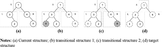
The topological reanalysis starts with expanding stiffness and factor matrices symbolically to that of transitional structure. Corresponding manipulation in the partition tree is attaching a blank sub-tree, as shown in Figure 7(a) to 7(b). After that element stiffness matrices are assembled to or dissembled from the stiffness matrix K of transitional structure. Then UMTF updates the factor matrices L and D from Figure 7(b) to 7(c). Finally, the stiffness and factor matrices are compressed to the target state. This corresponds to deletion of the blank sub-tree, as shown in Figure 7(c) to 7(d).
Detailed procedure from 6(b) to 6(c) consists of (1) mark the directly modified rows in transitional K as well as in L; (2) according to Rule 1, mark the affected rows in L; (3) update L using UMTF.
It is worth to note that other schemes such as “compression first and then expansion” can be implemented in a similar way with slight saving on storage space and computational effort. However, considering the program similarity, these schemes are not demonstrated in this paper.
4. Numerical examples and analysis
In this section, three examples are selected to show the accuracy and efficiency of the proposed topological reanalysis algorithm. Then, two examples from topological optimization and construction sequential analysis are adopted to show the capability of the algorithm in engineering problems.
4.1 Benchmark
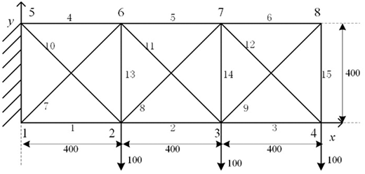
A truss structure with 15 bars subjected to three concentrated loads, as shown in Figure 8, is considered to verify the accuracy of the proposed topological reanalysis algorithm. The unit of dimension is mm, modulus of elasticity E is 3 × 10⁵ MPa and the cross-section area is 20.0 mm2. The truss structure is subjected to three steps of modification: Step 1 deletes elements 6, 9, 15 and the node 8; Step 2 adds elements 6, 9 as well as node 8 and deletes elements 3, 12 as well as node 4 (the concentrated force on node 4 is also inactive); Step 3 adds elements 3, 12, 15 and node 4 and back to the original structure.
Horizontal and vertical displacements of Node 3, 4, 8 (if active) by reanalysis algorithm and full analysis are listed in Table VIII. It is shown that the proposed topological reanalysis algorithm provides exact solutions as the full analysis.
Displacements result by reanalysis and full analysis (mm)
| DOF | Step 1 | Step 2 | Step 3 (original structure) | |||
|---|---|---|---|---|---|---|
| Reanalysis | Full analysis | Reanalysis | Full analysis | Reanalysis | Full analysis | |
| x3 | −0.044 | −0.044 | −0.018 | −0.018 | −0.044 | −0.044 |
| y3 | −0.150 | −0.150 | −0.073 | −0.073 | −0.152 | −0.152 |
| x4 | −0.051 | 0.051 | – | – | −0.048 | −0.048 |
| y4 | −0.263 | −0.263 | – | – | −0.251 | −0.251 |
| x8 | – | – | 0.016 | 0.016 | 0.045 | 0.045 |
| y8 | – | – | −0.106 | −0.106 | −0.249 | −0.249 |
As the proposed algorithm directly update the factor matrix without any approximation, the solution is supposed to be as accurate as a full analysis if round-off error is negligible. For simplicity, only efficiency of the algorithm will be concerned in following examples.
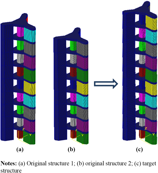
4.2 A large-scale building structure
A large-scale building structure is selected to show the capability of the proposed algorithm. The building has 200 floors and is composed of ten segments, as shown in Figure 9(c). The finite element model consists of 1,127,841 DOFs and 144,433 elements, and there are 75,907,479 non-zeros in the upper stiffness matrix and 672,195,675 in factor matrix after fill-in reduction. A full analysis of the entire structure involves 1,149,121.898 MFLOP (million floating-point operations). As the largest structure in this paper, the example is tested on Windows 10 system with Intel® Core™ i7-5820K (3.30 GHz) and 16GB RAM.
In each case, the original structure consists of a number of lower segments of the complete structure. The original structures are all modified to the target by addition of the rest segments. The first two of eight original structures are shown in Figure 9(a, b). In Table IX, after a row for reference data of full analysis of the target structure, added elements, added DOFs, number of operations and execution time for each modification as well as their ratio to the results of full analysis are given.
Results of reanalyzing large-scale building
| Case | Original segments | Added element | Added DOFs | Number of operations/MFLOP | Execution time/sec | ||||
|---|---|---|---|---|---|---|---|---|---|
| Full analysis | 144,433 | 1,127,841 | 1,149,121.9 | 299.6 | |||||
| 1 | 9 | 13,387 | 9.3% | 99,579 | 8.8% | 239,146.1 | 20.8% | 80.8 | 27.0% |
| 2 | 8 | 26,732 | 18.5% | 198,918 | 17.6% | 321,031.8 | 27.9% | 98.9 | 33.0% |
| 3 | 7 | 40,114 | 27.8% | 298,428 | 26.5% | 489,437.1 | 42.6% | 137.3 | 45.8% |
| 4 | 6 | 53,519 | 37.1% | 398,091 | 35.3% | 517,618.9 | 45.0% | 142.3 | 47.5% |
| 5 | 5 | 67,008 | 46.4% | 498,336 | 44.2% | 601,315.4 | 52.3% | 161.5 | 53.9% |
| 6 | 4 | 80,543 | 55.8% | 598,911 | 53.1% | 851,664.3 | 74.1% | 228.2 | 76.2% |
| 7 | 3 | 95,533 | 66.1% | 718,587 | 63.7% | 932,020.9 | 81.1% | 242.1 | 80.8% |
| 8 | 2 | 101,160 | 70.0% | 752,538 | 66.7% | 944,144.9 | 82.2% | 243.0 | 81.1% |
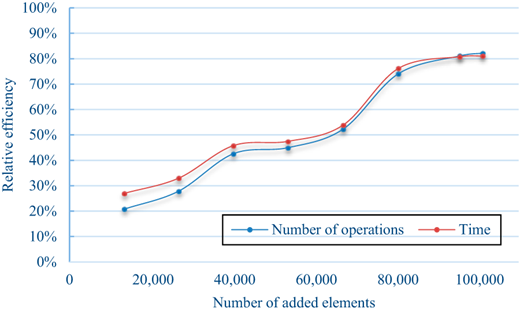
For the case of one segment addition, the added elements is 9.27 per cent of the target structure, and the proposed algorithm takes 20.8 per cent operations and 27 per cent computational time of the full analysis, which is a remarkable saving.
It is shown in Figure 10 that the execution time is proportional to the number of operations. As the added elements increase, the computational effort of the proposed reanalysis method grows not fast. When 53,519 elements, i.e. 37 per cent of the full structure, are added, only below 50 per cent computational operations and time of the full analysis is required, which shows the superiority of the reanalysis method for local high-rank modifications.
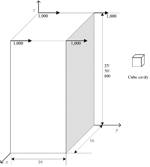
4.3 Cuboids with random local cavities
Three cuboids of size (1) 16 × 16 × 25, (2) 16 × 16 × 50, (3) 16 × 16 × 100 mm3, as shown in Figure 11, are used to show computational efficiency in different aspects. The bottom surface fixed cuboids are subjected to four concentrated forces at four corners of the upper surface. The Young’s modulus E is 210 GPa and Poisson’s ratio ν is 0.3. The cuboids are discretized into 13 cubes by 21-node solid elements. Table X lists the analysis information of the cuboids, where the last three columns give the numbers of nonzero entries in the upper triangular part of matrix K and U, as well as the computational effort by full analysis. The unit for computational effort is MFLOP (million floating-point operations).
Statistical data of the cuboids
| Cuboid | Dimension | Elements | DOFs | Non-zeros of upper K | Non-zeros of U | No. of operations/MFLOP |
|---|---|---|---|---|---|---|
| 1 | 16 × 16 × 25 | 6,400 | 103,350 | 7,962,909 | 94,475,526 | 194,441.9 |
| 2 | 16 × 16 × 50 | 12,800 | 206,700 | 16,104,684 | 223,241,601 | 605,623.2 |
| 3 | 16 × 16 × 100 | 25,600 | 413,400 | 32,388,234 | 493,859,301 | 1,546,239.2 |
In each sample, a cubic cavity of size varying from 13 to 103 is randomly created in the cuboid. For each cavity size, average computational cost of 50 samples at random locations are calculated to estimate the performance of the algorithm. Computational effort by the proposed topological reanalysis algorithm in comparison with full analysis are listed in Tables XI to XIII for cuboid (1), (2) and (3) respectively. It has been demonstrated in (Song et al., 2014) that the computational time required is generally proportional to the number of operations. This phenomenon is also supported by the example in 4.2 of this paper.
Computational effort for caving cuboid (1)
| Reanalysis/MFLOP | |||||
|---|---|---|---|---|---|
| Cavity size | DOFs (Modified) | Average | Mean variance | Full analysis/MFLOP | Operation ratio (%) |
| 13 | 103,347 | 84,737.6 | 3,094.2 | 194,441.9 | 43.6 |
| 23 | 103,300 | 87,473.94 | 9,738.2 | 194,315.7 | 45.0 |
| 33 | 103,112 | 89,193.34 | 11,107.8 | 193,454.8 | 46.1 |
| 43 | 102,726 | 99,455.38 | 22,004.5 | 190,485.0 | 52.2 |
| 53 | 101,987 | 92,668.29 | 13,469.1 | 186,491.7 | 49.7 |
| 63 | 100,874 | 94,985.97 | 21,388.3 | 179,060.5 | 53.1 |
| 73 | 99,253 | 10,2663.3 | 23,848.9 | 167,063.6 | 61.5 |
| 83 | 97,011 | 10,6038.6 | 28,176.4 | 152,090.2 | 69.7 |
| 93 | 94,205 | 96,096.52 | 28,923.9 | 138,051.5 | 69.6 |
| 103 | 90,366 | 98,561.63 | 28,522.0 | 118,423.1 | 83.2 |
Computational effort for caving cuboid (2)
| Reanalysis/MFLOP | |||||
|---|---|---|---|---|---|
| Cavity size | DOFs (Modified) | Average | Mean variance | Full analysis/MFLOP | Operation ratio (%) |
| 13 | 206,697 | 209,375.0 | 15,747.24 | 605,623.2 | 34.6 |
| 23 | 206,651 | 223,450.4 | 29,561.62 | 605,359.2 | 36.9 |
| 33 | 206,473 | 226,281.6 | 39,776.44 | 603,458.6 | 37.5 |
| 43 | 206,061 | 227,678.3 | 45,037.34 | 600,984.6 | 37.9 |
| 53 | 205,365 | 251,645.2 | 56,605.75 | 591,786.8 | 42.5 |
| 63 | 204,229 | 240,323.1 | 53,821.5 | 582,488.1 | 41.3 |
| 73 | 202,638 | 246,846.2 | 66,568.01 | 566,108.2 | 43.6 |
| 83 | 200,332 | 231,432.0 | 55,227.15 | 549,383.1 | 42.1 |
| 93 | 197,501 | 242,443.6 | 68,747.73 | 512,965.9 | 47.3 |
| 103 | 193,761 | 238,864.3 | 60,630.65 | 487,045.5 | 49.0 |
Computational effort for caving cuboid (3)
| Reanalysis/MFLOP | |||||
|---|---|---|---|---|---|
| Cavity size | DOFs (Modified) | Average | Mean variance | Full analysis/MFLOP | Operation ratio (%) |
| 13 | 413,397 | 386,197.6 | 36,229.11 | 1,546,239.2 | 25.0 |
| 23 | 413,349 | 388,691.7 | 36,394.56 | 1,545,990.6 | 25.1 |
| 33 | 413,171 | 407,282.4 | 80,316.59 | 1,544,252.0 | 26.4 |
| 43 | 412,771 | 413,420.5 | 79,405.57 | 1,539,175.0 | 26.9 |
| 53 | 412,055 | 416,646.6 | 61,746.12 | 1,530,919.5 | 27.2 |
| 63 | 410,923 | 417,409.9 | 82,381.38 | 1,519,585.7 | 27.5 |
| 73 | 409,310 | 434,935.6 | 88,563.34 | 1,496,454.4 | 29.1 |
| 83 | 407,075 | 425,499.9 | 70,021.42 | 1,470,869.5 | 28.9 |
| 93 | 404,241 | 420,599.3 | 10,0972.4 | 1,441,849.3 | 29.2 |
| 103 | 400,479 | 416,018.5 | 98,036.47 | 1,405,367.7 | 29.6 |
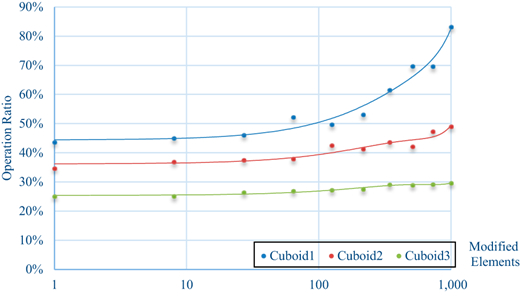
The numerical result indicates that, comparing with full analysis, the proposed algorithm presents a steady and remarkable operation saving for local modifications. For modification of one element deletion, the proposed algorithm takes average 43.6 per cent, 34.6 per cent, 25.0 per cent computational effort of the full analysis in three examples. As the size of modification growing, the ratio of the computational effort increases slowly. For modification about 2.50 per cent elements deletion, the computational effort ratios increase to 53.1 per cent, 42.1 per cent, 29.6 per cent respectively. It is shown that the proposed algorithm is efficient for local high-rank modification.
This property can be explained by Rule 2, that two adjacent elements usually exist in one subgraph in the partition tree and their modification paths are mostly overlapped. Therefore, addition of several elements in the same subgraph of the partition tree only brings a small portion of extra computational effort. However, once the modification stretches across different branches in the partition tree, the computational effort will show a sudden jump.
In addition, a higher efficiency is found in larger structures compared to smaller ones. With same size of cavity, the operation ratio in cuboid (3) is much less than the ratio in cuboid (2) and cuboid (1), as shown in Figure 12. This is because that the large-scale structure generally shows a stronger sparsity in both the stiffness matrix and factor matrix, which greatly influences the efficiency of the proposed algorithm. The proceeds of the proposed topological reanalysis usually grows as the problem’s scale increasing.
4.4 Applications in engineering problems
4.4.1 Evolutionary structural optimization.
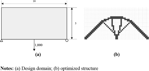
In this section, the proposed topological reanalysis algorithm is applied to evolutionary structural optimization (ESO) method (Zuo and Xie, 2014), which evolves the structure towards an optimum by slowly removing its inefficient material, to show the efficiency of the algorithm.
As shown in Figure 13(a), the design domain is a 5 × 10 m two-dimensional rectangular plate, with fixed support and simple support at each bottom corner and a concentrated force at the middle of the bottom side. The plate is discretized into 50 × 100 eight-node quadrilateral plane stress elements with The Young’s modulus E = 210 GPa and Poisson’s ratio ν = 0.3. The optimized structure is shown in Figure 13(b). The solution information is sampled every 1/10 of the whole optimization process. Numbers of floating-point operations of reanalysis algorithm and full analysis are listed and compared in Table XIV. The total operations by two approaches in the whole process are given at the end.
Computation effort of selected steps in optimization process
| Step | Element number | DOFs | Deleted element | Number of operation/MFLOP | ||
|---|---|---|---|---|---|---|
| Reanalysis | Full analysis | Ratio (%) | ||||
| 1 | 3,674 | 22,730 | 1,326 | 238.9 | 319.2 | 74.8 |
| 75 | 2,842 | 17,794 | 2 | 106.9 | 218.7 | 48.9 |
| 150 | 2,578 | 16,198 | 2 | 73.1 | 191.9 | 38.1 |
| 225 | 2,338 | 14,758 | 2 | 78.7 | 167.7 | 46.9 |
| 300 | 1,990 | 12,826 | 2 | 54.6 | 122.9 | 44.5 |
| 375 | 1,716 | 11,226 | 2 | 38.9 | 93.0 | 41.8 |
| 450 | 1,422 | 9,514 | 4 | 32.5 | 63.3 | 51.4 |
| 525 | 1,182 | 8,122 | 6 | 23.7 | 46.4 | 51.2 |
| 600 | 968 | 6,878 | 6 | 18.5 | 31.9 | 57.8 |
| 675 | 778 | 5,778 | 2 | 8.2 | 22.0 | 37.4 |
| 742 | 574 | 4,712 | 10 | 1.3 | 9.1 | 14.8 |
| Summation | 37,651.0 | 81,703.9 | 46.1 | |||
In the optimization process, successive modification are involved, and size and location of modification are determined by computations in each step. The result shows that the proposed algorithm effectively saves 53.9 per cent of the computational cost for solution of the entire process. At the beginning of optimization, modification is usually large and dispersed in separate areas, and the algorithm shows less effective. As shown in the first step, 1,326 elements are deleted because of a high initial rejection ratio. The modified elements accounts for 26.52 per cent of the entire design domain and disperse in four areas, and the computation savings of the algorithm is only 25.2 per cent. During the intermediate steps, the algorithm presents a comparatively steady performance. Because of symmetry of the problem, the modified elements are dispersed in two separate regions, which has a negative effect on the performance of reanalysis. It is noted that for bi-directional evolutionary optimization (BESO) which allows addition of elements, the reanalysis algorithm is also applicable.
4.4.2 Sequential construction analysis.
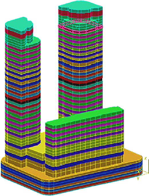
Sequential construction analysis (SCA) is a static analysis method for tall buildings. Comparing with the traditional model of one-time loading approach, SCA takes the mechanical properties that constructions are built and loaded level-by-level into account and reflects the structural response more accurately. In SCA, the intermediate structure in each step of the construction process need be solved. View one step of construction as topological modifications and then the reanalysis algorithm is applied to solve the similar structures in adjacent steps. In this section, reanalysis is applied to SCA in incremental direction which accords with the practical construction sequence.
SCA of a multi-tower building structure of 46 construction steps, as shown in Figure 14, is implemented. Structural information and computational effort of every nine steps are recorded in Table XV. The total operations by two approaches in the whole process are given in the last row.
Structural information and computational effort
| Construction step | DOFs | Modified elements | Number of operations/MFLOPS | ||
|---|---|---|---|---|---|
| Reanalysis | Full analysis | Ratio (%) | |||
| 9 | 166,191 | 2,898 | 20,603.9 | 33,172.5 | 62.1 |
| 18 | 259,440 | 2,870 | 24,087.9 | 73,245.3 | 32.9 |
| 27 | 313,596 | 1,861 | 17,128.9 | 93,052.5 | 18.4 |
| 36 | 367,857 | 1,935 | 18,360.5 | 117,987.9 | 15.6 |
| 46 | 442,683 | 1,236 | 28,442.2 | 143,484.1 | 19.8 |
| Summation | 814,279.9 | 3,684,817.0 | 22.1 | ||
The total floating-point operation number shows that algorithm has a good performance to multi-tower problems which cannot be solved by most present reanalysis methods. The proposed topological reanalysis algorithm makes a significant saving in the computation work, where the total saving rate is 77.9 per cent in this example. By comparing the performance between different steps, it is found that the algorithm generally brings more benefit as the problem scale increases.
5. Conclusion
The successive topological reanalysis arising in topology optimization, sequential construction analysis, etc., is a hard task in the sense that order of the resultant system of linear equations and value of matrix entries are changed simultaneously. In literature, general direct reanalysis approaches are not available. In this paper, we extended the updating matrix triangular factorization (UMTF) method to topological reanalysis by assuming an integral structure, which including all potential elements is introduced as a fundamental concept for data management of modified stiffness and factor matrix. The topological modification is divided into symbolic as well as numerical phase and processed separately. In addition, main data arrangement and an appropriate program flow is designed. By updating only the modified part of the factor matrix, the computational work is considerably reduced comparing with the full analysis. Examples show that the proposed reanalysis algorithm for topological modifications suits for a series of problems.
The proposed algorithm has several advantages, as follows:
It is applicable to general modifications with nodes/elements addition and deletion simultaneously in one step.
It keeps DOFs of the modified structures in a nearly fill-in optimized sequence during the whole modification process, and thus guarantees the efficiency of UMTF.
Compared to SMW-based algorithms, it explicitly updates in each step the triangular factor of the stiffness matrix so that performing for successive topological reanalysis is possible.
It allows both topological and non-topological modifications in one step.
It is based on the row-sparse solution framework and only requires a small amount of extra memory and has compatibility and capability for large-scale problems.
The major shortcoming is the requirement of locality of modifications in each step. The efficiency declines quickly when the modification is dispersed. Generally, the reanalysis is valid for modification distributed only in several regions but becomes inefficient for global modifications. In addition, because all potential elements included in the integral structure are supposed to be known, special problems such as adaptive elements generation cannot be solved.
The authors are grateful for the financial support received from National Key R&D Program of China (No. 2017YFC0803300) and NSFC Project (No. 11472014). The authors thank Mr. XL Wang from YJK software Ltd. who provided the data of examples.
