Evaluating energy performance of educational buildings: a case study in Australia

The operation of buildings approximately consumed 30% of global final energy demand and resulted in 26% of global energy-related emissions in 2022 (International Energy Agency, 2023). Commercial buildings, including educational buildings, were responsible for 32% of the final electricity consumption (Atalay et al., 2019). Shiel and West (2015) estimated that commercial buildings used half of the total energy used by buildings in the European Union and the USA. The authors further stated that 50% of this energy was used by heating, ventilation and air-conditioning (HVAC) systems to provide indoor thermal comfort. For commercial and educational buildings in Australia, HVAC is generally the largest end-use of electricity (43% of the total use), while space heating is the dominant user of gas (Department of Climate Change and Energy Efficiency, 2012). Growing urbanisation and prosperity are also expected to double the energy demand and carbon emissions in the building sector (Kc and Ruth, 2017). Therefore, it is important to understand building performance in terms of energy resources and end-use types to manage and optimise energy consumption in a building (Wei et al., 2018). Schito and Lucchi (2023) provided an overview of reducing building energy use, including improving the energy performance of building envelope, selecting efficient appliances, lighting and HVAC and utilising renewable and clean energy. Nardi and Lucchi (2023) also provided outlooks on in situ thermal transmittance assessment of building envelope, including the emerging techniques used for the U-value measurement and the potential use of AI and data-driven methods for the U-value retrieval or assessment.

Previous research related to building energy use performance can be classified into residential and non-residential categories. Residential studies consist of a single or group of houses (Fumo and Rafe Biswas, 2015; Li et al., 2016; Chen et al., 2018; Li et al., 2017), while non-residential energy performance studies encompass a single or a group of commercial, industrial and educational buildings (Lam et al., 2010; Martani et al., 2012; Shiel and West, 2015; Kc and Ruth, 2017; Tang et al., 2025). Some energy-efficient buildings, such as zero energy buildings (ZEBs), typically use less energy than traditional buildings. The concept of ZEBs was proposed in the 1970s (Papadopoulos, 2016) and ZEBs are characterised by their total energy consumption equal to zero for a given period (Belussi et al., 2019). To achieve ZEBs, one of the main aspects should be addressed, namely energy savings in building services, including HVAC systems, hot water and lighting (Aljashaami et al., 2024). For example, Tejani et al. (2022) proposed an investigation into the application of HVAC systems in the conceptualisation and realisation of ZEBs and the use of effective operational techniques in the enhancement of energy efficiency. Kazmi and Oca (2016) improved the energy efficiency of domestic hot water provision operations for ZEBs. When dealing with the issue of ZEBs, it is essential to know their exact energy consumption patterns. The energy consumption patterns in buildings can be impacted by several factors, including climate, energy costs, availability of natural resources, local and national energy policies, technological development and social and cultural factors (Zhang et al., 2021).

To analyse the energy performance of buildings, Shiel and West (2015) examined the influence of external temperature on building energy use and the accuracy of prediction models, as the authors considered that the most important predictor of energy use in commercial buildings is the external temperature. In addition, the researchers also observed that the daily average temperature is generally a good predictor of building energy consumption. However, it may not be applicable in all cases. Hence, they introduced a parameter called Natural Thermal Lag to incorporate the differences in outdoor and indoor temperature to help increase the accuracy of energy use prediction models.

Furthermore, Chen et al. (2018) employed a segmented linear regression approach to calculate electricity-temperature sensitivities for 1,245 households across California. The authors endeavoured to mainly find the impact of the spatiotemporal resolution of selected datasets on the calculated relationship between residential electricity consumption and ambient temperature. They found that using different temperature indicators (hourly, daily minimum, daily average and daily maximum) significantly affected the R² value of the regression between temperature and calculated electricity-temperature sensitivity. The overall hourly relationship showed weaker coefficients than daily metrics, and among the daily indicators, daily average temperature versus electricity use showed the highest coefficient compared to the minimum and maximum temperatures. In addition, Fumo and Rafe Biswas (2015) used simple and multiple linear regression analysis to examine the nature of the relationship between energy consumption and parameters such as outdoor temperature and solar radiation in a single-family residential building. The authors observed that adding solar radiation as a second predictor variable improved the coefficient of determination, but the root mean square error was reduced, which showed the importance of both variables in ensuring the quality of models. Li et al. (2016) conducted a linear regression analysis of the energy used for space heating and temperature setpoints and concluded that they are well-fitted with a coefficient of determination (R²) of 0.995. Li et al. (2016) also conducted linear regression between energy consumption and two variables, including indoor-outdoor temperature difference and working/non-working day, with an R² value of 0.892.

As discussed above, regression models and time series analysis have been commonly used in the analysis of energy consumption for buildings. In order to forecast energy consumption from climate variables such as temperature, Geng et al. (2018) used a multiple-parameter regression model based on monthly energy bills and weather data to find the relationship between outdoor air temperature and energy use in an office building in China. The coefficients obtained from the regression between monthly average energy use and outdoor air temperature were used to estimate the energy used for the HVAC system and other uses such as lighting, plug and auxiliary systems. Furthermore, the actual energy use of the HVAC and others was compared with that of simulated energy uses as benchmark data. In 2019, Atalay et al. (2019) developed and assessed the performance of statistical methods such as multiple regression analysis, time series and Grey models to estimate the electricity consumption of the HVAC system of a commercial building in France using weather variables. They found that outdoor temperature was the dominant parameter that influenced the HVAC electricity consumption, and relative humidity had an insignificant influence on the same. The authors further stated that multiple linear regression analysis provided the most effective model for predicting HVAC electricity consumption. Gunay et al. (2018) developed models that predicted the frequency of custom set point temperature change requests in four large office buildings using multivariate logistic regression models and concurrent indoor and outdoor temperature records. In 2021, Mohammed et al. (2021) proposed a regression-based model for predicting the energy consumption of one of the most significant energy-consuming types of facilities in Saudi Arabia: schools. Their model utilised 350 actual data points of energy consumption collected from schools operating in the eastern province of Saudi Arabia. A sensitivity analysis indicated that important factors affecting energy consumption were air conditioner capacity and building age. Yang et al. (2022) employed a multiple linear regression model to predict the electricity consumption of buildings located at a university in Xiamen, China, based on the investigation of the daily electricity usage data of 8 apartment complexes. Using a linear regression analysis based on RETScreen Version 9, Udisi et al. (2025) indicated the 80% correlation between the building's natural gas consumption and the Heating Degree Days.

The studies on the energy consumption of schools and universities mainly focus on the campus as a whole or only a certain kind of building (Wei et al., 2022). Generally, university and school buildings have some unique features in terms of their occupancy profiles, which are highly variable within small time intervals when compared to other buildings, making it important to study the energy use profiles at various time steps (Martani et al., 2012). However, the studies that exclusively investigated the energy use of educational buildings are limited. Martani et al. (2012) used a new approach of using WiFi connections as a proxy for occupancy in an educational building at the Massachusetts Institute of Technology in the US to study the influence of human activity on energy use. The results demonstrated that the energy use associated with HVAC systems was mostly influenced by factors like external temperature rather than occupancy levels, while occupancy caused changes in small levels of electricity use. Kc and Ruth (2017) attempted to understand the influence of outside temperature on electricity consumption in institutional buildings (Northeastern University, USA) by performing multiple linear regressions and deriving heating and cooling degree days. They found that the increase in one cooling degree day caused an increase of 0.124 kW/m² in electricity use, whereas it was 0.025 kW/m² for an increase of one heating degree day in winter. Ma et al. (2017) also studied building-related energy use, focussing on university buildings. They used a new approach called variation-focused cluster analysis strategy to identify daily heating energy profiles in 19 university buildings. The outcomes from this study provided insights into peaks and troughs of daily heating profiles and helped to categorise buildings with similar use profiles.

In addition, Im et al. (2022) investigated the impact of climate change on a university campus' energy use and revealed that the equipment power density is an important factor for electricity consumption, while the heating degree is a critical factor for steam consumption. Moghayedi et al. (2024) investigated that green methods and technologies may result in improved resource efficiency in educational buildings in South Africa. In 2025, a university building in Beijing was selected as a case study. Tang et al. (2025) mentioned factors impacting energy consumption by reviewing existing literature, and established a framework for illustrating the interactions between the identified factors, such as social and economic factors. The electricity consumption was also analysed in a representative sample of thirty schools in Manitoba, Canada (Ouf et al., 2016). The research found that, though the total gas consumption for heating decreased in the new school, the total electricity consumption showed a significant increase, which might be due to the use of more complex HVAC systems, including programmable thermostats. In addition, a descriptive statistical method was also developed to reveal the energy use profiles of 35 university buildings in Norway (Guan et al., 2016). It was observed that the electricity use was influenced by occupancy levels, while seasonal factors affected the heating energy more. The literature survey shows that there is a need to investigate the energy use characteristics of educational buildings due to their unique occupancy levels and there is an increased interest in assessing the energy use performance of educational buildings and understanding the underlying causes of variation in consumption. In Australia, Khoshbakht et al. (2018) investigated the characteristics of energy use in different types of buildings on higher education campuses. The authors aimed to establish an energy benchmark system through the analysis of energy consumption and energy use intensity, as well as related space types and occupancy conditions. Gui et al. (2020) then evaluated the impacts of different space uses on energy use in terms of buildings from 5 university campuses. The study demonstrated that wet laboratories use a large amount of energy because of their energy-intensive equipment and high requirement for mechanical ventilation. The data in the above-mentioned research is mainly derived from educational buildings in subtropical Australia and analysed at the building level. The study of Tavakoli et al. (2023) focused on electricity consumption and COVID-19 effects on this consumption in office buildings of an Australian university. The results reveal that a change in the load profile of a building due to a lockdown highly depends on the purpose of the building. It is imperative to understand the energy performance of educational buildings in different climates and at various temporal scales. Moreover, energy-saving potentials need to be further explored in Australia within this context. For example, energy uses of educational buildings, including electricity and gas, need to be extensively investigated for space heating and cooling, DHW heating, lighting and other power usage in Australia. It is also worthwhile to identify the potential relationships between energy use and outdoor temperatures for Australian educational buildings.

Due to the increased concern about carbon emissions and resource use by the building sector, the building industry is focussing on designing sustainable buildings. Many new buildings have been constructed in recent years, following the best design practices as stipulated by rating agencies in respective regions to achieve sustainability. These buildings are designed in such a way that both capital and operating resource use, mainly energy, water and materials, are claimed to be sustainable in nature, which contributes to lower carbon emissions. Ouf et al. (2016) observed that new and green buildings with sustainability design features could be 25–30% more energy-efficient than conventional buildings, but indicated that some new buildings consumed more electricity than conventional ones. Geng noted that there was a performance gap between the design stage and operation stages of a building and confirmed that this gap makes it difficult to predict or control building energy consumption. Therefore, it is imperative to analyse the operational performance of the building to identify causes for poor performance, especially the energy use at various temporal scales. This will provide quality feedback to facility managers, builders and users about the actual performance of the building and target specific items to reduce/optimise resource usage. Furthermore, a better understanding of energy use and its relationships with weather factors, especially outdoor temperature, helps to reduce the uncertainties related to building performance and guide efficiency improvements. Based on the above insights, this study will assess the energy use performance of an educational building using monitored data at various temporal scales using an integrated approach combining monitoring data, regression modelling, psychrometric analysis and validation. This study will also explore the extent of energy-saving potentials while maintaining indoor thermal comfort through psychrometric analysis. Thus, this study provides novel contributions by offering multi-scale insights into the energy use dynamics of Australian educational buildings.

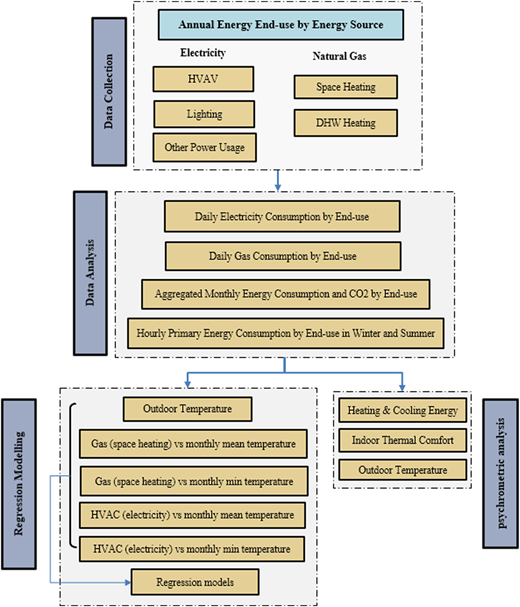
This research examines the actual energy performance using monitored data and explores energy-saving potential using an Australian education building as an example. As illustrated in Figure 1, the research methodology comprises data collection, data analysis, regression modelling and psychrometric analysis through a case study. (1) Annual energy end-use by energy source (electricity and natural gas) is collected for HVAC, lighting, other power usage, space heating and DHW heating for the studied building. (2) The collected data are analysed by the energy source and end-use at various temporal scales, including daily electricity and gas consumption by end-use, aggregated monthly energy consumption and CO₂ emissions by end-use and hourly primary energy consumption by end-use during winter and summer. (3) Furthermore, regression modelling is conducted between gas (space heating), HVAC (electricity) and outdoor minimum and mean temperatures. Researchers considered that regression analysis is capable of providing a more significant indications of the dispersion and correlation of data (Tahmasebinia et al., 2023) and also offers advantages such as ease of use, interpretability and so on (Pino-Mejías et al., 2017). Thus, data regression is explored to identify potential relationships in this paper. (4) Based on the analysis, energy saving potential is explored through psychrometric analysis.

The Centre for Advanced Design in Engineering Training (CADET) building, illustrated in Figure 2, is an advanced educational facility at Deakin University, Victoria, Australia. Completed in 2015, this three-level facility spans 8,512 m² and houses the School of Engineering. The building features advanced systems, engineering laboratories and learning spaces, providing practical educational experiences for engineering and design students.

Critical to its energy performance, the building employs several passive design strategies. The building envelope incorporates high-performance double glazing, metallic insulated roof panels and perforated metal screens on the western glazing to control solar radiation while maintaining thermal performance and daylight. A central chimney on the roof enables passive ventilation and cooling in summer, while thermal mass strategies, such as concrete floors and walls, provide passive heating and cooling. The building's HVAC system is designed to optimise energy performance. The system features an air-cooled chiller, highly efficient gas-based condensing boilers and zoning for heating and cooling. Secondary and passive approaches, including slab heating, external shading, crossflow ventilation, night-time purging and chilled beams, reduce the energy load on the system. A thermal wheel in the air-handling unit transfers 85% of the exhaust air heat to the incoming air, further reducing energy consumption. The HVAC system's design and components contribute to reducing energy use, operational costs and carbon emissions. The building's energy consumption is primarily driven by three main components: the HVAC system for cooling, lighting and other power systems, including standby electrical equipment and lab equipment.

Energy consumption data for electricity, natural gas and water were collected from metres installed throughout the building. The data were recorded and stored in the Climate Change Action Plan (CCAP) integrated reporting tool provided by Kinesis, an advanced urban analytics and modelling platform. This platform integrates diverse datasets from various metres within a building or precinct, presenting them in a unified manner to facilitate analysis of resource usage performance. To ensure data reliability, we employed a rigorous validation process. Automated validation checks were conducted to identify and address potential outliers or missing data points. We also compared the data collected from CCAP with manually downloaded data from metres as a process of data comparison and validation for the case building.

The raw data for electricity, water and natural gas consumption in the building were available at 15-minute intervals for 2018. The choice of the year was due to data availability, with recent years (2019–2024) having data interruptions, while the 2018 dataset provided a comprehensive and uninterrupted record of energy consumption, allowing for a thorough analysis of the building's energy performance. We justified this choice by ensuring that the data were representative of typical building operations and that any anomalies or interruptions were adequately addressed. The collected data were categorised into three main end-uses: HVAC, lighting and other power systems. The HVAC sub-metres measure only the electricity used for ventilation and air conditioning, mainly for cooling. The energy needed for space heating primarily came from natural gas, with some electricity used for fans and pumps (included in HVAC metre readings). Two sub-metres were installed to measure natural gas consumption individually for space and water heating. Based on the monitoring data, the overall energy consumption can be derived and categorised as follows:

where $ECT$ represents total energy consumption (kWh); $EHVAC$ is the electricity used for HVAC (kWh); $EHeatingG$ is the natural gas consumption used for space heating (kWh); $EDHWG$ is the natural gas used for DHW heating (kWh); $EL$ is the electricity used for lighting (kWh); $EO$ is the electricity used for other purposes (kWh), such as equipment and appliances.

In this study, the electricity and natural gas data for the calendar year 2018 (January to December) were considered on an hourly, daily and monthly basis for various analyses. The 2018 dataset provided a sufficient timescale to analyse energy consumption patterns. The HVAC electricity data in kWh from various sub-metres in the building were initially combined to observe the total building HVAC electricity consumption. Similarly, lighting and other end-use data were aggregated for the entire building. As the HVAC electricity use data were identifiable for each level, level-wise use data were also consolidated. The natural gas data for space heating and water heating were available in terms of m³. To enable a comparison between the energy used by space heating and other end uses, the gas usage in m³ was converted to equivalent kWh using the calorific value of gas supplied in the study region.

To examine average hourly trends of energy use, hourly data from January (summer) and July (winter) were analysed for weekdays and weekends. Trends were observed for both weekdays and weekends, along with standard deviations. Natural gas volume in m³ was converted to equivalent electricity use in kWh per hour for comparative analysis between end-uses. Monthly patterns of energy use by the HVAC system, heating, lighting and other uses were analysed by examining the monthly average daily electricity uses. Average daily carbon emissions in kgCO_2-e were calculated for each month using Equations (2) and (3) to assess environmental sustainability trends throughout the year. Carbon emission factors for electricity and natural gas consumption were obtained from Scope 3 greenhouse gas (GHG) emissions (Environment Protection Authority Victoria, 2022). To normalise the data and facilitate meaningful comparisons, we calculated the energy consumption per unit area (kWh/m²) per annum. This approach enabled us to identify trends and patterns in energy usage and to evaluate the building's performance against key performance indicators and the National Australian Built Environment Rating System (NABERS) rating.

Where: $CO2−eG$ is CO₂ emission of natural gas (kg); $CO2−eE$ is CO₂ emission of electricity (kg); $V$ is the gas volume (m³); $EFG$ is the emission factor of natural gas (kg/m³); E is electricity consumption (kWh); $EFE$ is the emission factor of electricity (kg/kWh).

Outdoor air temperature is the most direct weather variable that affects the seasonal component of electricity use in a building, as found by several past studies (Fumo and Rafe Biswas, 2015; Shiel and West, 2015; Kc and Ruth, 2017; Geng et al., 2018; Li et al., 2017), though other variables such as solar radiation, heating and cooling degree days could also be used. Furthermore, many of these studies pointed out the influence of temperature on electricity use by HVAC systems. Regression analysis is one of the most widely accepted statistical approaches for assessing the relationship between electricity consumption and weather variables, especially outdoor temperature (Lam et al., 2010; Fumo and Rafe Biswas, 2015; Thornton et al., 2016; Li et al., 2017; Atalay et al., 2019). As this study aims to analyse the association between a single predictor variable, i.e., the outdoor temperature and heating and cooling energy consumption (response variables) in a building, a simple linear regression was used here. Separate linear regressions were carried out for HVAC (electricity) and gas (space heating) to find the correlation of the two variables with temperature. Minimum, mean and maximum outdoor temperatures were regressed against HVAC (electricity) and gas (space heating) use to identify the extent of association at a monthly temporal scales. The temperature data for the year 2018 were obtained from the Australian Bureau of Meteorology for the nearest weather station.

In order to identify energy-saving potentials, psychrometric analysis is conducted using a design tool named Climate Consultant 6^® developed by the UCLA Department of Architecture and Urban Design (The Society of Building Science Educators, 2023) in this research. Climate Consultant translates raw climate data into meaningful graphic displays, representing the attributes of climate and its impact on building design. In particular, the psychrometric chart produced by the tool illustrates the impacts of different design strategies on indoor thermal comfort. Therefore, this tool was used in this study to find sustainable building design strategies, which would help optimise indoor thermal comfort, thereby minimising energy consumption for heating and cooling. Within Climate Consultant, the comfort model of ASHRAE standard 55 was chosen to represent the indoor thermal comfort of the building with the centralised HVAC system. This standard specifies the combinations of various factors, including environmental and personal factors, that result in satisfactory thermal conditions for most occupants. The model provides criteria for evaluating comfort in existing buildings, as well as requirements and calculation procedures for design compliance (ASHRAE, 2023).

The temperature range within which forced or mechanical heating/cooling was not required to keep the indoor conditions at comfortable levels was noted. This was used to estimate the electricity that could be saved if the building was designed according to the best design strategies as given by the tool. Climate data for Melbourne were used as input data in the tool, as this was close to the study building, with a similar mild temperate climate (Australian Building Codes Board, 2019). The following sections report and discuss the results obtained in this study.

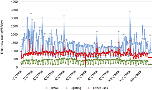
The daily electricity consumption of the building by end-use for the year 2018 is shown in Figure 2. The average electricity consumption for HVAC, lighting and other power usages are 1,345 kWh/day, 378 kWh/day and 841 kWh/day, respectively. The HVAC system consumes 52% of the total power energy.

It can be seen from the figure that the HVAC electricity use was showing a seasonal trend, while electricity for lighting and other power usages remained almost constant, except for weekdays and weekends. As mentioned in Section 2.1, electricity consumption for the HVAC system mainly included ventilation and air conditioning during warm periods and therefore, the electricity use peaked during the months of January and February, as those are the months with recorded maximum temperature during the year. The electricity consumption again increased during the last two months of the year, according to the rise in temperature. The average weekday HVAC electricity use during the first three months of the year was 1,988 kWh/day, while it was 1,628 kWh/day for April and May, which are transition months. The average electricity use was the lowest, 1,331 kWh/day, during the colder months, starting from June and extending until the shoulder month of October. The electricity use climbed to an average weekday value of 1,612 kWh/day during the remaining period of the year. The average daily HVAC electricity use during weekends was 779 kWh/day, which shows that a considerable amount of energy was spent when the occupancy levels were supposedly low.

The average daily electricity use for lighting during the weekdays was 457 kWh/day, while it was 218 kWh/day during the weekends. The same for other uses were 887 kWh/day and 741 kWh/day, respectively. It can be noted that the difference between average weekday and weekend electricity demand for other uses was smaller than that for HVAC and lighting. This could be due to standby electricity use by appliances such as computers, large audio-visual screens, lab equipment and kitchen appliances.

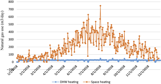
The daily consumption of gas for space heating and water heating over 2018 is shown in Figure 3. As in the case of HVAC electricity use, the gas consumption for space heating clearly showed a seasonal pattern. The space heating energy consumption peaked during the middle of the year, which was the winter months and decreased gradually towards the summer period. The average total gas use in 2018 was identical at 218 m³/day, and the average gas use for space heating was 197 m³/day. The average gas use for space heating was the minimum from January to March at around 60 m³/day, while it was maximum from June to September at around 341 m³/day. Thus, the average gas use during the winter months was more than five times that of the summer period.

However, from the figure, the gas used for heating water in the building was relatively constant throughout the year except for a few spikes and dips. The average gas use for water heating in 2018 was identical at 24 m³/day. Hot water is mainly used in faucets in the kitchen, common areas and toilets. The gas use trend for water heating illustrates that it was not affected by seasonal changes. Even the trend during weekdays and weekends was very similar, with an average daily gas use of around 25 m³/day for weekdays and 23 m³/day for weekends. Thus, the volume of gas, or in other words, the average energy required for space heating, was more than eight times that required for water heating in the building.

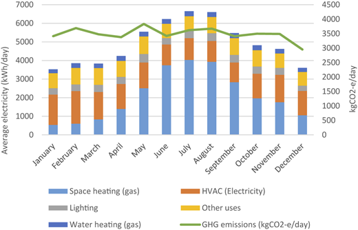
The average daily contribution of each end-use to the total energy consumed in the building across the months is shown in Figure 4. It is clear from the figure that, except for the first three months of the year, space heating energy use dominated the total energy consumption in the building. From May to September, the equivalent average daily electricity use for space heating was more than or equal to 50% of the total electricity use. There is a similar trend in the UK, as illustrated in the work of Thornton et al. (2016), in which a higher proportion of gas was consumed for heating compared to electricity. Moreover, this is true for most EU-15 countries (except for Spain, Portugal, Italy and Greece), where average electricity demand showed a single peak during winter months (Hekkenberg et al., 2009; Psiloglou et al., 2009). In countries like Spain, Portugal, Italy and Greece, there was an additional peak during the summer months (Hekkenberg et al., 2009; Psiloglou et al., 2009). In this study, the peak in average energy use occurred during winter, followed by transition months and the least use occurred in summer. In absolute terms, the average daily gas use for space heating in the case study building during the winter months of June, July and August was around 4,000 kWh/day. Overall, space heating dominated the total energy use of the building in the winter season.

When combined, the energy used by space heating and the HVAC system always contributed 60%–80% of the total energy use of the building. This is consistent with the findings of Lam et al. (2010) in China, where winter heating and summer cooling accounted for 65% of the energy use in the building sector. Though the absolute electricity use values remained almost similar for lighting, other power usages and water heating, the percentage contribution by each of them was reduced by the middle of the year and the spring months. The stable values of lighting, other power usages and water heating throughout the year indicate that heating and cooling should be the main targets for implementing energy conservation measures in the building. The share of total energy used by water heating varied between 4.1% and 6.8%. This is contrary to what Nair et al. (2018) observed in an academic building in Ireland, where 30% of the total building energy use was contributed by water heating during the winter months. However, Pérez-Lombard et al. (2008) noted that in the US and UK office buildings, water heating accounted for about 4% and 10% of the total energy use, respectively, which is closer to the value found in this case study.

In Figure 3, the monthly average daily GHG emissions contributed by the total energy use in the building are also illustrated in terms of kgCO_2e. The emissions ranged from 2,952 to 3,834 kgCO_2e per day across the months, with an average of around 34,880 kgCO_2e. The average carbon emission intensity of the study building in 2018 is equivalent to around 150 kgCO_2e/m² per year and was much lower than the average annual carbon emission intensity of Victorian university buildings as of 2011, which was around 285 kgCO_2e/m² (Department of Climate Change and Energy Efficiency, 2012). It is interesting to note that the GHG emission was not the highest during the winter months, though the energy use was at its maximum. This was due to the increased use of natural gas for heating, which has lower carbon emissions per unit of energy than electricity. The highest carbon equivalent emission was observed in May, and the lowest in December. The carbon emission trends may change once the campus microgrid becomes fully operational and starts supplying electricity to the building.

It is difficult to compare and rank large non-residential buildings, especially tertiary educational institutes, based on their energy use sustainability. Several factors, such as purpose, occupancy levels, type of HVAC system and electrical equipment used and their efficiency levels, make the difference. However, energy use per unit floor area is one metric widely used to report the energy intensity of buildings. In this case, the energy intensity of the building during 2018 was found to be 211 kWh/m² per annum. Using data from 2003 to 2010, the Department of Climate Change and Energy Efficiency (2012) estimated that the average energy intensity for university buildings in Australia had increased from 217 kWh/m² in 2001 to 241 kWh/m² in 2011, and university buildings in Victoria were found to be the most energy-intensive at over 306 kWh/m² on average per annum between 2001 and 2011. Thus, the energy intensity of the case study building in 2018 was less than the national and the 2011 Victorian average. According to the City of Melbourne, new offices having more than 2,000 m² of gross floor area should at least have a 5-star NABERS rating (Seo et al., 2014) and their planning scheme requires the projected energy intensity for new commercial buildings should be 64 kWh/m² in 2021 and 60 kWh/m² in 2026 as set by the city of Melbourne.

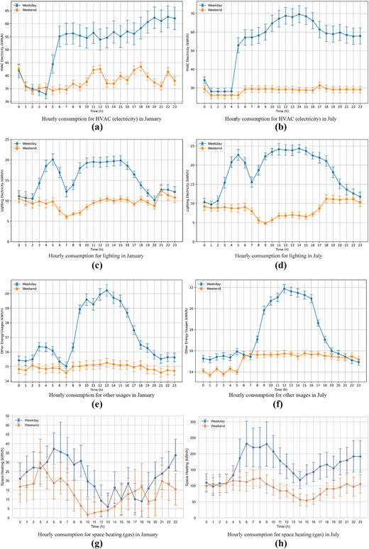
The hourly energy consumption trends of various end-use in a typical summer and winter month are given in Figure 5. The average hourly energy use patterns for weekdays and weekends in January and July 2018 are plotted against 24 hours to understand the dynamics of energy use on a finer temporal scale. Standard deviations in each plot show the variation in energy consumption from the mean during each hour. The left pane shows the hourly consumption plots during January, while the plots on the right side indicate July trends.

Figures 5a and 5b show the average hourly HVAC electricity use on weekdays and weekends during January and July 2018. The electricity use in January has higher deviations from average values than in July for both weekdays and weekends. The electricity use was found to be minimal during the early hours of the day (1:00 am to 4:00 am) in both months, when weekdays and weekends had a similar usage rate. The hourly electricity consumption associated with lighting in January and June is illustrated in Figures 6c and 6d. The difference between weekday and weekend profiles was greater during January than in July, when the trends were almost similar. In January and July, the lighting electricity use varied between 5 kWh/h and 25 kWh/h, and there was a reduction in electricity use at 7:00 am for both weekdays and weekends in January.

Figures 5e and 5f depict the hourly trend of electricity consumption for other end uses in common spaces and labs in the building. It is interesting to note that the electricity use was almost constant for weekends in both January and July. There was a clear rise in energy use from 8:00 am to 6:00 p.m. in both January and July. The identical weekend profiles indicate that there was a requirement for standby/base electricity of around 15–16 kWh/h in the building, whether or not it was operating. The natural gas used for space heating on an hourly basis for January and July is shown in Figures 6g and 6h. As January was the warmer period, the space heating energy requirement was obviously lower than that in July. The average hourly gas use peaked around 5–6 am in both January and July, with 35–40 kWh/h during the weekday in January and 200–250 kWh/h in July. The deviations from mean values were higher in January. When comparing the electricity used by HVAC with the gas used for space heating, more energy per hour was expended for heating in a typical winter period than for cooling in a typical summertime.

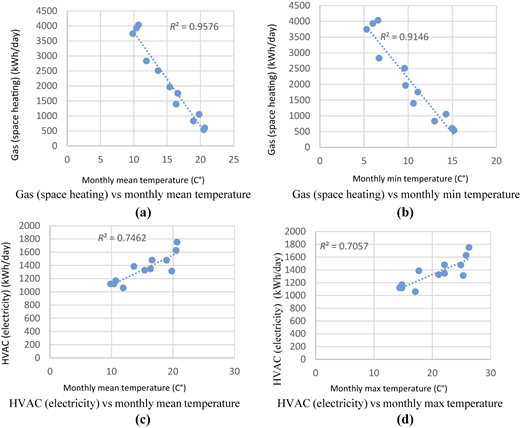
To assess the effect of temperature on the cooling and heating energy requirements in the building, the outdoor temperature is regressed against HVAC electricity and gas use, as shown in Figure 6. The sub-plots show the relationships between mean, minimum and maximum outdoor temperature against monthly average daily energy use.

Figures 6a and 6b show the regression of monthly average daily heating energy use against mean and minimum temperature. The coefficient of determination (R²) was found to be slightly greater for heating versus mean temperature compared to heating versus minimum temperature. Therefore, energy consumption and temperature showed the strongest correlation when regressed using energy data at monthly temporal resolution and using mean temperature, which is expressed using Equation (4). The correlation level between temperature and heating and cooling electricity consumption in buildings varies from place to place according to climatic conditions. For example, a study conducted by Kc and Ruth (2017) using data from 26 buildings in Northeastern University, Boston in the US found that summer months had a greater influence of outdoor temperature on electricity use, followed by transition months and winter. A similar outcome was observed by Pagliarini et al. (2019) in Milan, Italy, from 2013 to 2017, where electricity use during summer had greater sensitivity to outdoor temperature than that in winter. However, in a country like the UK, where the summers are mild, the daily electricity and gas demand have a strong negative correlation with temperature (Thornton et al., 2016). In addition, Thornton et al. (2016) found that winter electricity and gas demand had the strongest anti-correlation with temperature compared to other periods. More studies with similar objectives and temporal and spatial resolutions are required to make effective comparisons and benchmarking between buildings in different climatic zones and geographical regions.

where $EDG$ is the natural gas consumption used for space heating (kWh/day); $TO$ represents outdoor monthly mean temperature (°C).

Sub-plots 6c and 6d illustrate the relationships between monthly energy use for HVAC (electricity), and mean and maximum outdoor temperatures. It can be seen that the temperature indicator (mean or maximum) selected could affect the R² value. The mean temperature was found to have a slightly higher impact on electricity use. The possible reason could be the high temporal fluctuation of maximum temperature over a year as compared to the mean temperature. From the sub-plots 6c to 6d, the trend of the fit line indicates a positive coefficient of correlation between temperature and HVAC electricity use and therefore, electricity use increased because of the temperature increase.

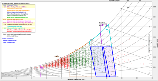
This section discusses the energy savings potential of adopting optimal design strategies for thermal comfort in the studied building. The software Climate Consultant 6 (The Society of Building Science Educators, 2023) was employed to determine the best design approaches to maintain indoor comfort while minimising electricity use. The program suggested strategies based on the nearest meteorological data, and their effectiveness is illustrated in the psychrometric chart (Figure 7). The chart displays the comfortable temperature range (green dots) and the non-comfortable areas (red dots) when the proposed strategies are adopted.

Alternatively, the modelling recommendations imply that energy expenditure on heating and cooling between 14°C and 26°C could be reduced by employing building design strategies that incorporate energy-saving features, such as internal heat gain, passive solar direct gains, high thermal mass and sun shading of windows. Figure 7 suggests that the internal heat gain from lights, occupants and equipment contributes 3,552 comfortable hours (40.5% of the annual hours), which can be achieved through insulation and air tightness of the building envelope. Figure 7 also illustrates that passive solar heating through window glazing and high thermal mass contributes 1,342 comfortable hours (15.3% of the annual hours). Furthermore, sun shading of windows contributes 368 comfortable hours (4.2% of the annual hours). While these options represent new building designs, they could potentially save about 8.9% of energy demand by encouraging occupants to dress appropriately for their own thermal comfort.

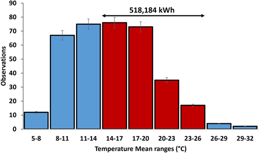
Figure 8 depicts the distribution of heating and cooling energy usage within the studied building across different outdoor temperature ranges. The dark red bars represent observations of energy usage occurring between 14°C and 26°C, which account for approximately 518,184 kWh of annual electricity usage. On the other hand, the blue bars are observations of energy usage occurring outside the temperature range of 14°C and 26°C. To calculate the potential energy savings, we divided the saved energy by the total energy consumed and multiplied the result by 100 to express it as a percentage. This yielded a potential for saving 42% of the total annual energy by implementing the recommended design strategies.

However, it is important to note that retrofitting existing buildings, such as the case study building, may present certain trade-offs and limitations. Factors like air gaps, insulation inadequacies and high air turnover may require additional heating or cooling, thus reducing energy conservation potential. Despite these challenges, the modelling outcomes offer valuable insights into the energy-saving possibilities of ideally designed buildings that modify or filter external climatic conditions to establish indoor thermal comfort.

The literature shows that there is an increased interest in assessing the energy use performance of educational buildings and understanding the underlying causes of variation in consumption. However, limited research has been conducted on educational buildings in Australia within this context. This study analysed the energy use performance of a relatively new educational building featuring green design and sustainable building practices in Australia to inform the energy usage trends at various temporal scales. The correlation between various temperature indicators and electricity use at different temporal scales, as well as the effect of thermal comfort levels on electricity use, were investigated to obtain insights about the building.

The energy intensity of the whole building was found to be 211 kWh/m² per annum (January–December 2018), less than the national and the 2011 Victorian average, though short of future targets (60 kWh/m²). The results from this study also highlighted the seasonality of heating and cooling systems in the building, in contrast to more stable energy uses, such as lighting and water heating. More energy was expended on building heating in a typical winter period than on cooling in a typical summertime. This trend is similar to that of building energy use in most northern European countries with mild climate zones. A similar trend is also observed by Thornton et al. (2016), namely a higher proportion of gas consumed for heating compared to electricity, when observing the equivalent average daily electricity use from May to September. When combined, the energy used by space heating and the HVAC system always contributed between 60% and 80% of the total energy use of the building. This result is consistent with the findings of Lam et al. (2010) in China, where winter heating and summer cooling accounted for 65% of the energy use in the building sector. Similarly, the energy use for heating has reached the largest proportion of all end-use categories for the operation of residential buildings in Victoria (Stephan, 2013), as winters are severe in Victoria (Strategies, 2008). Thus, improving the energy efficiency of the heating system is an effective way to reduce operational energy in Victoria and improving the thermal insulation of the ceiling, wall, floor and glazing reduces operational energy. Another effective way to reduce energy use is to raise building occupants' awareness of energy conservation and encourage them to take energy-saving actions. The supply-side solutions could include the application of renewable energy (e.g. solar PV system, solar thermal water heater and ground source heat pump system) as the energy source for academic buildings.

Unlike the academic building in Ireland, 30% of the total building energy use was contributed by water heating during the winter months Nair et al. (2018). The share of total energy used by water heating varied between 4.1% and 6.8% in the CADET building. However, this result is consistent with the findings of office buildings provided by Pérez-Lombard et al. (2008) in the US and UK. Water heating accounted for about 4% and 10% of the total energy use, respectively. The hourly energy consumption trends of various end-use in a typical summer and winter month were analysed in this research, and the patterns were compared between weekdays and weekends, providing the dynamics of energy use on a finer temporal scale.

When using linear regression models, this case study showed a positive correlation between temperature and HVAC electricity use, while temperature and gas used for space heating showed a strong negative correlation. Moreover, the regression involving gas used for space heating in winter demonstrated a stronger correlation with temperature than HVAC electricity in summer at the monthly temporal resolutions. Using the tool Climate Consultant 6, the best design strategies for providing internal thermal comfort were visualised. Though the tool is not building-specific and there may be discrepancies due to local influences, it was estimated that there was a potential for saving around 42% of the total annual building electricity, provided the design strategies are followed. The ideal building design strategies that would enable energy-saving measures are internal heat gain, passive solar direct gains, high thermal mass and sun shading of windows.

Understanding building energy use is crucial for reducing energy consumption and mitigating climate change. This study meticulously evaluated the energy use of a campus building in Australia using monitored data, providing insights at various temporal scales to understand the dynamics of energy use. The key findings are as follows: the studied building performed more efficiently than the national and state averages, with an annual energy use intensity of 211 kWh/m², although it fell short of Melbourne's future target of 60 kWh/m²; the building produced 150 kg CO₂-e/m² per year, significantly lower than the average annual carbon emission intensity of Victorian university buildings in 2011 (285 kg CO₂-e/m²); more energy was consumed for space heating in winter than for cooling in summer; hourly energy consumption trends for various end-uses in typical summer and winter months illustrated distinct patterns between weekdays and weekends; the regression analysis showed a strong correlation between space heating in winter and outdoor temperatures; and the psychrometric chart analysis identified potential energy savings of around 42% of the total annual building electricity while maintaining indoor thermal comfort.

As a part of making the campus carbon-neutral by 2030, the university is currently establishing a renewable energy microgrid. It consists of a 7 megawatt (MW) centralised solar farm on 14.5 hectares and 0.25 MW rooftop solar generation systems on existing buildings, including the building. The grid construction and connection have just been completed at the time of writing this article, and soon, it is expected to supply around 54% of the campus's current power consumption. This will reduce 12,000 tonnes of GHG emissions per year at the campus. The findings from this study will, therefore, form an important baseline to help stakeholders evaluate how the microgrid changes building energy use and emissions and to identify areas for improvement to achieve carbon neutrality. Furthermore, the microgrid can contribute to the non-space heating component of the energy requirement of the building and it would greatly reduce the carbon emissions emanating from conventional electricity (mostly generated from coal) use. This could be achievable as the peak electricity use for cooling occurs during summer months, and this coincides with the highest energy generation potential of solar PV.

In addition, to facilitate the implementation of energy-efficient measures, researchers, building managers, policymakers and energy professionals should consider the following implications: (1) implementing continuous monitoring systems to track energy use patterns in real-time, enabling proactive management and quick response to inefficiencies. (2) designing buildings that optimise energy use across different seasons, incorporating passive design strategies and utilising advanced analytics to inform energy management practices. Passive design strategies align with the principles of sustainability by reducing the use of non-renewable resources and minimising the environmental impact of the building. (3) training building occupants to ensure better building operation. An effective way to reduce energy use is to raise building occupants' awareness of energy conservation and encourage them to take energy-saving actions. Therefore, providing guidance to users can ensure the efficient operation of the energy system in academic buildings.

This study provides novel contributions by offering multi-scale insights into the energy use dynamics of Australian educational buildings through a case study and identifying energy-saving potential through passive design strategies based on psychrometric analysis. Based on high-frequency monitoring data, the energy uses of the educational building, including electricity and gas, are extensively investigated for space heating and cooling, DHW heating, lighting and other power usage. It also identifies the relationships between energy use and outdoor temperatures for the Australian educational building. Furthermore, psychrometric analysis investigates potential energy savings while ensuring indoor thermal comfort through passive design strategies. This research also analyses high-frequency monitoring data, which can be used to benchmark similar buildings in the region and guide improvements toward achieving net-zero energy targets. This study enriches the global research on the energy performance of educational buildings through multi-scale data analysis, a case study and the psychrometric analysis of energy-saving potential.

While this study contributes significantly to the understanding of building energy use, it is not without limitations. The analysis is restricted to data from 2018 due to data interruptions between 2019 and 2024, and future studies should incorporate more recent data to validate these findings and account for any changes in building performance over time. While the ASHRAE Standard 55 model provides a robust framework, certain limitations and assumptions entailed in ASHRAE Standard 55 might affect the generalisability of our findings. For example, variations in human occupancy and activity levels, which can significantly impact thermal comfort, were averaged in ASHRAE Standard 55. While the research focus of this paper is to address the energy performance of a specific educational building as a case study, it is worthwhile to compare the performance and relevant models for buildings across different regions and climate conditions in future research. Furthermore, we propose collecting other variables, such as the number of occupants, the number of electronic devices and the operating time of these devices, to develop sophisticated models to predict the energy performance of educational buildings in future research. The study's scope could also be expanded to explore the impact of occupant behaviours on energy use, the effectiveness of different energy-saving technologies and design strategies identified using Climate Consultant based on thermal comfort models and the scalability of these findings to other building types and regions.