


Existing classifications of inflationary regimes often rely on subjective judgments, hindering objectivity and accuracy. This study proposes a novel, data-driven approach to address this limitation.
We combine unsupervised clustering and classification tree methods to analyze Argentine inflation data from 1943 to 2022. Two smoothing techniques are introduced: a measure of temporal contiguity and a rolling majority rule method. The resulting regimes are compared to existing classifications based on their explanatory power for inflation-relative price variability.
Our method identifies distinct inflationary regimes, demonstrating significant improvement in objectivity and accuracy compared to existing literature. The regimes capture key historical periods and exhibit a strong association with inflation-relative price variability, providing valuable insights into Argentine inflation dynamics.
This study offers a novel methodological framework for constructing objective and accurate inflationary regimes, free from subjective biases. This approach holds potential for application to other contexts and contributes to a more nuanced understanding of inflation dynamics.
List of abbreviations
1. Introduction
Despite inflation being one of the most relevant topics in Economics, various aspects regarding its characterization have been vaguely explored by the literature. In particular, the notion of an “inflationary regime”, despite its extensive use, is based on subjective criteria without an existing consensus among researchers. This is problematic since is not independent of value judgments and is potentially subject to bias and classification errors.
Different alternatives were proposed in the literature regarding the number of inflationary regimes and the limits that define them, without reaching a consensus. In general, these characterizations are associated with the definition of numerical thresholds (Bruno & Easterly, 1998; Cagan, 1956; Dabús, 2000; Dornbusch, Sturzenegger, Wolf, Fischer, & Barro, 1990; Dornbusch & Fischer, 1993; Werner & Bazdresch, 2000), except Heymann and Leijonhufvud (1995), who rely on the behavior of the agents. Furthermore, due to their general construction, these classifications do not capture the heterogeneity inherent to the inflationary processes of each country but rather generalize a set of inflationary regimes for all of them.
The objective of this work is to introduce a new methodological approach that uses machine learning techniques for the characterization, classification, and periodization of inflationary regimes in Argentina. Our goal is to improve the methodological aspects of this procedure relative to the current literature. By doing so, we seek to enhance the analysis of macroeconomic data, reduce the subjectivity in the research process, and capture the unique aspects of the country. Argentina’s extensive history of inflation makes it an ideal case to study, as it enables us to identify the different inflationary regimes that are commonly used.
We use the k-means algorithm to construct the inflationary regimes and calculate their threshold values using classification and regression trees (CART), following the work of González and Delbianco (2021) and Levy-Yeyati and Sturzenegger (2005) who used clustering techniques to study the history of MERCOSUR and the development of exchange rate regimes, respectively. Then, we internally validate the obtained clusters by performing ANOVA analysis and silhouette analysis.
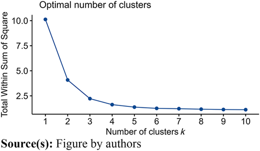
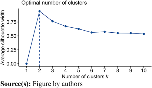
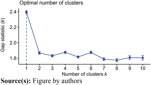
The distinctive nature of inflation data (in particular, the presence of outliers) makes commonly used methods for selecting the optimal number of clusters, such as the Elbow Method or the Gap Statistic, unsuitable in this context. Therefore, we opt to present the results for four regimes arbitrarily. Additional results for three and five clusters are provided in Appendix 2.
Due to the nature of the problem under study, it is necessary to smooth the classification obtained over time. For this purpose, we introduce a new measure called Temporal Contiguity Distance (TCD), which modifies the distance between observations according to their temporal proximity. This improves clustering over time by making it more likely that two adjacent observations belong to the same cluster. Alternatively, we also introduce a rolling procedure that applies the simple majority voting rule within a time window. This approach assigns the prevailing regime within the window to each observation. We also examine the performance of the different regimes proposed regarding the relationship between inflation and relative price variability, comparing our analysis to that conducted by Dabús (2000) and Caraballo, Dabús, and Usabiaga (2006). Finally, we apply our methodology to inflation in Brazil and the United States to illustrate how outcomes may differ based on each nation’s inflationary history.
This paper makes several contributions. Firstly, we contribute to the literature on the intersection of macroeconomics and machine learning by presenting a less arbitrary data-driven characterization of inflationary regimes specific to Argentina’s inflationary history. Furthermore, we propose new regimes that perform better in explanatory power than those present in previous studies. Additionally, we contribute to the clustering literature by introducing two novel procedures that incorporate the temporal dimension of data, enabling a smoother classification over time. This approach makes it easier to interpret and analyze historically and can have broader applications in other contexts.
The proposed approach is useful mainly for two reasons. On the one hand, classifying inflation periods into different regimes is essential for gaining a nuanced understanding of economic conditions and formulating effective monetary and fiscal policies. On the other hand, a country-specific inflationary regime classification offers the advantage of precision and customization, allowing policymakers and stakeholders to address the unique challenges faced by individual economies. This tailored approach enhances the effectiveness of economic policies and promotes better-informed decision-making. The methodology is then suitable for adaptation and use in different economies and periods.
The rest of the work is structured as follows. Section 2 presents a literature review of different definitions and characteristics of inflationary regimes. Section 3 addresses the methodological approach to be adopted and the sources of information. Section 4 shows the estimates of the regimes, the historical periodization of Argentine inflation, the comparison with previous studies for the inflation-relative prices variability relationship, and the results for Brazil and the United States. Finally, Section 5 concludes.
2. Literature review
There are various criteria to classify inflation, one of the most used is to categorize it into different regimes based on the rate at which prices increase for a certain temporal unit (Frisch, 1984).
Cagan’s research on the dynamics of hyperinflation constitutes one of the earliest contributions on the subject (Cagan (1956)). The author defines the beginning of hyperinflation when prices increase at least 50% per month (12,875% annually) and its end when it remains sustained below that threshold for at least a year.
Nevertheless, various authors proposed alternative definitions for hyperinflation. For example, Dornbusch et al. (1990) in their study on extreme inflationary episodes reject Cagan’s rule, using a lower threshold for hyperinflation of 1,000% per year (implying monthly rates above 15 to 20%, sustained for several months).
For Kiguel (1989), hyperinflation is an intrinsically unstable process that countries can experience even at levels lower than the 50% proposed by Cagan. In this sense, Dornbusch (1992) points out that the distinction between hyperinflation and cases of extreme but slightly lower inflation is arbitrary because the behavior of the economy between these levels is virtually identical, with inflation as the dominant factor of the economy. Under this conception, in a subsequent study, Kiguel and Liviatan (1995) relaxed Cagan’s rule to correctly delimit the end of the Peruvian hyperinflation of 1988–1990. This allowed them to analyze the non-explosive dynamics that the episode exhibited. Additionally, the authors characterize a high inflation regime at rates between 20 and 49% monthly (792–11,874% annually).
An alternative criterion is provided by Bruno and Easterly (1998), who in their study of high inflation crises consider a threshold of 40% annually for at least two consecutive years to classify such episodes. This limit is determined based on the observation of a break in the economic dynamics close to that value, from which inflation tends to accelerate and become more volatile, increasing the probability of leading to hyperinflation.
In contrast to these studies, there is the characterization provided by Heymann and Leijonhufvud (1995), who propose inflationary regimes in terms of the planning horizon of the agents, expressed in which time unit the inflation rate is reported. In this way, inflation is moderate when individuals express it in annual terms, high when this horizon becomes one month, and hyperinflation when it is less than a month. The authors provide an approximate range of 5–50% per month for the high inflation regime, while agreeing with Cagan (1956) for hyperinflation.
Concerning moderate inflation, Brunner, Fratianni, Jordan, Meltzer, and Neumann (1973) characterize it as a state in which prices grow at annual rates rarely above 10%, with decelerations after relatively high inflationary peaks and with the possibility of some deflationary episodes. Along the same lines, Werner and Bazdresch (2000) study the dynamics and transitions of the moderate inflation regime (10–20% annually) to the low inflation regime (<10%) and the high inflation regime (>20 %). Conversely, Dornbusch and Fischer (1993) specify it at rates between 15% and 30% annually, for at least three consecutive years. Finally, Dabús (2000) in its study for Argentina, characterizes moderate inflation when monthly inflation is below 2%, high between 2 and 10%, very high between 10 and 50%, and hyperinflation for values greater than 50%, which makes it consistent with Cagan’s rule.
As can be noted, there is no consensus in the literature about the number of regimes or the limits that define them. This is a result of the arbitrariness of these definitions, which was already acknowledged by several of their authors (Bruno & Easterly, 1998; Cagan, 1956; Dornbusch, 1992; Werner & Bazdresch, 2000). With the exception of Bruno and Easterly (1998), these characterizations are not based on objective criteria or statistical methods; instead, they are grounded in the very inflationary processes that were intended to be analyzed, in value judgments, or in conventions that Economics has adopted over time, such as Cagan’s rule.
Recently, several authors employed threshold autoregressive models to determine regimes. In these studies, regimes are defined based on the search for breaks in the economic relations of interest, such as the relationship between inflation and relative prices (Bick & Nautz, 2008), or inflation and exchange rate pass-through (Brufman, Trajtenberg, & Donaldson, 2017; Cheikh & Louhichi, 2016; Costa & Ruffo, 2019). The limitation of these procedures is that the obtained regimes are not independent of the relationship of interest under study.
Along the same lines, Castagnino and D’Amato (2008) and D’Amato and Garegnani (2013) use structural change tests to identify breaks in an autoregressive process of Argentine inflation, characterizing the regimes based on the results of these tests. However, it is relevant to highlight that the authors conceive these regimes in a broader sense than usual, referring to monetary regimes that imply a particular institutional framework of economic policy.
A relevant feature captured by autoregressive models is that the dynamics of the economy and prices are different under different levels of inflation due to changes in the behavior of economic agents and price formation mechanisms. Several authors have studied the inflation-relative prices variability relationship, finding the presence of breakpoints in the dynamics between variables for different regimes (Caraballo et al., 2006; Dabús, 2000; Elias, Legnini, & Lliteras, 1996). In general, higher inflation is more volatile (Taylor, 1981) and is associated with greater price dispersion (Moll, 2017; Tommasi, 1992). This is explained by the stability of moderate inflation episodes reinforced by mechanisms such as indexation. On the other hand, hyperinflation exhibits unstable and explosive dynamics that can lead to a substantial economic decline. Regarding this, Bruno and Easterly (1998) presents evidence of a negative relationship between economic growth and inflation for high inflation crises.
In addition to the inherent characteristics of different regimes, they exhibit substantial variations between countries. These differences arise from the different public perceptions of inflation, the shocks that originated the inflationary process, the previous inflationary history, and other specific features of the economic structure that influence price dynamics. An example is the hysteresis effect, which consists of persistent low demand for local currency caused by a history of high inflation (Dabús, Delbianco, & Fioriti, 2016).
These differences can be observed in the high inflation and hyperinflation processes in Latin America during the 1980s, which present substantial differences from the European experiences of the 1920s. The former lasted longer, exceeding a decade, with relatively lower levels of inflation and a stop-and-go pattern, marked by temporary stabilizations followed by inflationary bursts (Dornbusch et al., 1990). On the other hand, European hyperinflations were triggered by external factors such as war, while in Latin America these were secondary, with domestic factors being the primary causes (Dornbusch, 1992). Kiguel and Liviatan (1995) attributes these differences to the prolonged history of high non-explosive inflation experiences in Latin America, which allowed small economic shocks to destabilize the economies and drive them towards hyperinflation.
In particular, Argentine hyperinflation showed similarities in duration and intensity with European experiences, while there were significant discrepancies in the fiscal domain. The prolonged inflationary history in Argentina resulted in greater government control and indexation mechanisms, which helped avoid the collapse of tax revenues seen in European hyperinflation (Kiguel & Liviatan, 1995). In the latter, the hyperinflation was attributed to a sudden and substantial increase in the fiscal deficit, whereas in Argentina, it originated from a prolonged process of deterioration of public accounts.
For Argentine inflation, it is also possible to identify distinctive features that separate it from the other experiences in Latin America. The strong influence of inflationary inertia is a characteristic that differentiates it from the rest of the region. In particular, the persistence of inflation is the factor that explains its variability to a greater extent, representing 80% of the inflation volatility for the period 2004–2019 (García-Cicco, Garegnani, Aguirre, Krysa, & Libonatti, 2023).
These distinctive features of inflationary regimes can be summarized in the following definition. Following Tohmé, Dabús, and London (2005), an inflationary regime is defined as an economic context characterized by an inflation rate fluctuating in a particular range of values, with a specific degree of uncertainty and a system of expectations associated. This definition understands each regime as a distinct pattern of connections in the economy, associated with a specific state of the economic system. Each of these states results in inflationary episodes of varying magnitude in accordance with past experiences and economic policy shocks. We consider this definition the most precise and complete, using it as a guideline for our analysis. It enables us to capture the notion that each economy will exhibit different regimes and operate differently depending on its current regime and duration. Therefore, it inclines us towards a country-specific approach, allowing for different regime classifications for countries with distinct inflationary histories. Furthermore, understanding the regimes as specific states of the economic system encourages us to prioritize smooth classifications over time and to develop procedures to ensure such outcomes.
From this review arises the need to improve the methods to identify the thresholds of different inflationary regimes, considering the heterogeneity of countries and the characteristics of each regime. This is where the use of machine learning methods becomes relevant, as they will enable, with minimal assumptions, to characterize, classify, and periodize inflation in an optimal way into distinct inflationary regimes specific to Argentina.
3. Data and methodology
3.1 Classification procedure
Because we do not start from a previous classification of regimes in the literature, it is necessary to use a procedure that endogenously generates the different categories along with their respective thresholds. An approach applied in the symbolic analysis literature is to select the threshold that minimizes the normalized Shannon entropy (Brida & Garrido, 2011). Another alternative is to segment the variable space by dividing it into subsets of values above and below their respective means (Brida, London, Punzo, & Risso, 2011; Cayssials, González, & London, 2022). This latter approach has limitations, as the mean may not be a representative threshold of the dynamics between regimes.
In their work, Caraballo et al. (2006) formulated a two-stage classification of inflationary regimes. Firstly, they conducted a periodization by searching for breaks in a smoothed inflation series. Secondly, they assigned a regime to each given period based on its average inflation rate, utilizing the regimes presented in Dabús (2000). Nonetheless, this approach has certain drawbacks, such as the requirement for a prior classification of inflationary regimes and the inability to identify smooth transitions between regimes.
In this work, we employ clustering techniques commonly used to identify patterns and structures in the data. These methods group observations into clusters based on their similarity, using a metric such as the Euclidean distance. The clusters are composed of units that are the most similar to one another, in comparison to those belonging to other clusters. We later interpret these groups as inflationary regimes.
Specifically, we use the k-means algorithm, which partitions the set of observations into k clusters, with each observation belonging to a unique cluster. This algorithm iteratively obtains an optimal partition by minimizing the Euclidean distances between the observations of the same cluster and its center, defined as the mean of the observations belonging to that cluster (Kassambara, 2017).
In comparison to other clustering techniques, such as hierarchical methods, this method excels in this type of problem as it requires minimal intervention from the researcher regarding the classification criteria employed (Levy-Yeyati & Sturzenegger, 2005). Additionally, its sensitivity to outliers, which in other contexts is problematic, is an advantage since it allows the hyperinflation regime to be correctly identified and isolated in the data. Alternatives such as k-medians or hierarchical methods present difficulties in this sense, erroneously assigning observations in the clusters. On the other hand, researchers have employed k-means in similar contexts where the goal was to reduce the arbitrariness of existing classifications. González and Delbianco (2021) use this method to obtain a historical periodization of MERCOSUR based on foreign trade indices, while Levy-Yeyati and Sturzenegger (2005) apply it to construct a classification of de facto exchange rate regimes based on the behavior of foreign exchange market variables.
Using clustering as our main methodology helps uncover hidden patterns and structures in inflation data, which can be useful for exploratory data analysis. By grouping similar data points, clustering can effectively reduce the dimensionality of data, making it easier to visualize and analyze in contrast to other economic series or periods.
Nevertheless, clustering techniques are highly sensitive to the data used, often resulting in unstable outcomes when the sample changes. Consequently, as new inflation data is gathered, the clustering results may differ, requiring careful consideration by researchers (Hastie, Tibshirani, Friedman, & Friedman, 2009).
There are two additional potential issues with clustering methods. First, some algorithms assume that clusters are spherical or convex, which may not be suitable for all datasets and can result in poor clustering results. Second, some clustering algorithms have high computational complexity, making them impractical for large datasets or real-time applications. However, these issues do not apply to inflation data, as assuming convexity is appropriate, and the time series are not large enough to pose computational complexity problems.
The presence of outliers in the sample, such as hyperinflationary episodes, disrupts the criteria for determining the optimal number of clusters. As a result, indicators suggest in favor of constructing two groups that manage to separate these observations from the rest of the sample (see Appendix 1). However, this approach would not allow us to capture the regimes that exist at lower levels of inflation. Moreover, factors such as the incorrect separability of clusters and significant differences in sample sizes, both elements that appear in this context, can compromise the efficacy of the gap statistic (Tibshirani, Walther, & Hastie, 2001; Yin et al., 2008). These reasons lead us to arbitrarily decide the number of clusters, which is a major shortcoming of this analysis. We opt to identify four inflationary regimes: low inflation, moderate inflation, high inflation, and hyperinflation. One could argue in favor of building the clusters by leaving aside extreme observations of hyperinflation or deflation to fix the issue mentioned above, but doing so would introduce more arbitrariness into the procedure, which goes against the purpose of this work. In Appendix 2, we present the results for three and five clusters for comparison.
We employ the CART tree-based classification method to determine the thresholds of the generated regimes. This technique uses the groups obtained by k-means as input and builds a decision tree that predicts them, recursively partitioning the variable space using optimal cutoff values (Breiman, Friedman, Stone, & Olshen, 1984; Murphy, 2012). The selection is based on a criterion that minimizes impurity of the classification in each node generated by the partitions (i.e. Gini impurity for this classification). These limits defined in terms of the variables constitute the thresholds of the inflationary regimes. Finally, to establish whether we forced a grouping of the data, the clusters obtained are internally validated through the analysis of variance (ANOVA) and the silhouette analysis.
CART can capture nonlinear relationships between features and the target variable, does not require assumptions about the underlying data distribution, and is invariant to different scaling (Hastie et al., 2009). These characteristics make it suitable for classifying inflation data. However, it is prone to overfitting, especially with noisy data or when the tree grows too deep. This issue can be mitigated by pruning or setting a maximum tree depth, which adds complexity. In this context, CART serves as an auxiliary method to delimit regime thresholds, while the main task of classification is performed by k-means, ensuring that overfitting is not a relevant issue.
3.2 Periodization
To achieve an effective historical periodization, a desired aspect would be that the assigned regimes exhibit smoothness over time, i.e. there should not be abrupt regime changes that are reversed in short periods. The utilization of monthly data in this study introduces a complication in this sense, whereas in prior research, employing annual data for cluster analysis alleviated the issue. To date, clustering techniques can account for the spatial contiguity of observations to achieve better grouping (Quintana, 2021), but no methods have been developed that consider temporal contiguity to group observations of time series.
To address this limitation, we present a new measure called Temporal Contiguity Distance (TCD) [1], based on re-weighting the Euclidean distance between observations according to their temporal proximity. The TCD aims to incorporate the temporal dimension into cluster analysis. It allows smoothing clustering over time because it increases the original distances as the observations move away in time, reducing the probability that they belong to the same cluster. Hence, two consecutive observations in a time series will receive a minimum increase in their distance, while for the first and last observations, the increase will be the maximum possible.
Formally, consider a matrix X of dimension (T × p), with p variables followed over T periods in time (t = 1, 2, …, T), and let λ be a non-negative real number. For a given λ, the TCD between two observations t and s is defined as:
The parameter λ regulates the temporal smoothing. When the value of λ equals zero, we obtain the original Euclidean distance, while larger values cause the Euclidean distances to grow at most by a factor of 1 + λ. Moreover, dividing by the maximum possible distance, T − 1, normalizes the factor to the temporal scale of the data.
To apply k-means with the TCD, it is necessary to transform the TCD matrix into a representation in the space of the p variables because k-means cannot be applied over a dissimilarity matrix. We achieved this through non-metric multidimensional scaling, which provides an optimal representation that best fits the dissimilarity matrix. Subsequently, k-means is applied to this transformed matrix. According to De Luca and Zuccolotto (2011), this two-stage procedure presents superior performance compared to the direct application of hierarchical methods to the dissimilarity matrix, as demonstrated through simulations.
An alternative strategy for smoothing the classification over time involves employing a voting rule where each observation acts as a ”voter” and casts a vote based on its associated regime. We apply this rule in a rolling time window on the series of regimes obtained by k-means. We opt for the simple majority rule for our voting mechanism, but it is worth noting that other voting rules or a different approach (e.g. assigning the median or the mode of the time window) could be used instead. The constructed procedure takes a time window from the observation t to h lags, within which the different assigned regimes are counted. Therefore, the voting interval has h + 1 observations. If a regime passes the simple majority rule, it is assigned to observation t. It is worth clarifying that at all times, voting is done based on the original data without considering previous votes. The following diagram provides a more detailed presentation of the procedure:
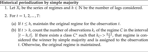
As an example, Table 1 illustrates the periodization for a series of 10 data points and a time window with 2 lags.
Example of periodization by simple majority
| t | Xt | Xt (simple majority) |
|---|---|---|
| 1 | Low inflation | Low inflation |
| 2 | Moderate inflation | Moderate inflation |
| 3 | Moderate inflation | Moderate inflation |
| 4 | Low inflation | Moderate inflation |
| 5 | Moderate inflation | Moderate inflation |
| 6 | High inflation | High inflation |
| 7 | Hyperinflation | Hyperinflation |
| 8 | Moderate inflation | Moderate inflation |
| 9 | Low inflation | Low inflation |
| 10 | Moderate inflation | Moderate inflation |
Source(s): The authors
Following the proposed steps, the first two observations remain unchanged, as well as those in which a simple majority winning regime does not result (t = 6–9). This guarantees that the series is smoothed in periods of relative stability where sporadically a regime change may have been identified (t = 4), while the results are not affected in intervals of high economic instability characterized by several regime changes(t = 6–9).
3.3 Data
Our sample comprises inflation data for the period between February 1943 and December 2022 inclusive. Due to various constraints, we use the monthly headline inflation rate as the sole variable for generating the clusters. Specifically, we were unable to create indicators of relative price variability due to a lack of complete historical data for disaggregated good categories of the Consumer Price Index between 1943 and 1989. Also, we were unable to incorporate inflation expectation indicators into our analysis due to a lack of data for the entire sample. Therefore, we have relied solely on monthly inflation rates as a classification variable without being able to consider other aspects of the dynamics of each regime.
The official inflation statistics from the National Institute of Statistics and Censuses of Argentina (INDEC) were manipulated and falsified by the national government between 2007 and 2015, resulting in underreported inflation rates (Miranda-Zanetti, Delbianco, & Tohmé, 2019). Due to this, we collected data for the period 1943–2006 and 2016–2022 from the Consumer Price Index of INDEC, while for the period 2007–2015, we used inflation data extracted from the inflacionverdadera.com website of the Billion Prices Project (Cavallo & Rigobon, 2016). This website employs online retail price data to construct inflation indexes for Argentina, which were in line with local estimates.
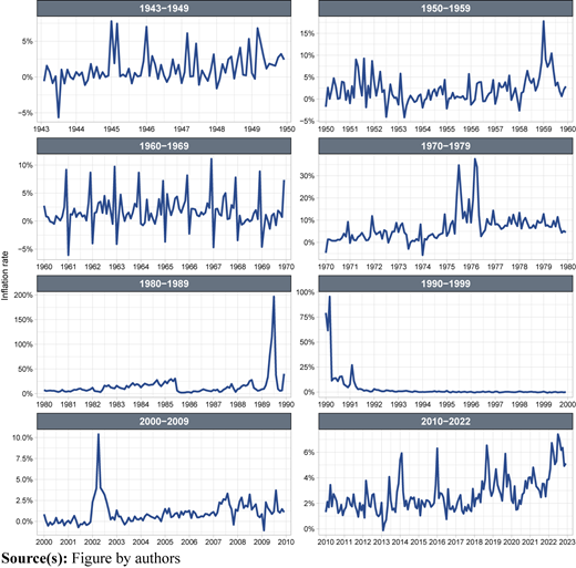
Table 2 provides the summary statistics for the monthly inflation rate, segmented by decade, while Figure 1 illustrates the corresponding time series for each period. These provide a comprehensive overview of Argentina’s inflationary history. Until 1980–1989, the two most severe inflationary episodes were in 1959 and 1975, the latter originated from an economic adjustment known as the “Rodrigazo”. The decade 1980–1989 was characterized by the highest inflation and significant instability, culminating in episodes of hyperinflation in 1989 and 1990. This period was subsequently followed by a decade of price stability, driven by the disinflation from the implementation of the Convertibility Plan.
Summary statistics of inflation by period
| Period | Mean | SD | Min | Max |
|---|---|---|---|---|
| 1943–1949 | 1.20 | 2.17 | −5.64 | 7.79 |
| 1950–1959 | 2.14 | 3.18 | −4.20 | 17.76 |
| 1960–1969 | 1.68 | 2.88 | −6.07 | 11.10 |
| 1970–1979 | 6.65 | 6.62 | −5.72 | 37.57 |
| 1980–1989 | 14.60 | 21.64 | 1.70 | 196.63 |
| 1990–1999 | 3.57 | 12.93 | −0.75 | 95.53 |
| 2000–2009 | 1.00 | 1.36 | −1.08 | 10.39 |
| 2010–2022 | 2.72 | 1.44 | −0.12 | 7.41 |
Source(s): Table by authors
4. Results
4.1 k-means estimations
Table 3 presents the results of the k-means estimation for the four regimes, along with the thresholds obtained through CART, which constitute intervals closed by their minimum and open by their maximum.
Cluster-level descriptive statistics
| Regimes | Obs. | Average | SD | Thresholds | |
|---|---|---|---|---|---|
| Inflation | Min | Max | |||
| Low inflation | 738 | 1.36 | 1.69 | – | 5.02 |
| Moderate inflation | 175 | 8.66 | 2.73 | 5.02 | 16.60 |
| High inflation | 41 | 24.30 | 8.92 | 16.60 | 70.02 |
| Hyperinflation | 5 | 112.86 | 49.08 | 70.02 | – |
Note(s): The numbers correspond to monthly inflation rates
Source(s): Table by authors
The results show a great preponderance of the low inflation regime, which constitutes more than 75% of the total sample of months. Also, the thresholds obtained exhibit higher values concerning those presented in the literature review, as shown in Table 4. For example, in contrast to the definition proposed by Cagan (1956) that considers hyperinflation starting at 50%, our results establish that the transition towards said regime occurs from a threshold of 70%.
Literature comparison
| Authors | Inflationary regimes | ||||
|---|---|---|---|---|---|
| Low | Moderate | High | Very high | Hyperinflation | |
| This paper | <5% | 5–17% | 17–70% | >70% | |
| Cagan (1956) [m] | – | – | – | – | >50% |
| Dornbusch et al. (1990) [m] | – | – | – | – | >15–20% |
| Kiguel and Liviatan (1995) [m] | – | – | 20–49% | – | >50% |
| Heymann and Leijonhufvud (1995) [m] | – | – | 5–50% | – | >50% |
| Dabús (2000) [m] | – | <2% | 2–10% | 10–50% | >50% |
| Brunner et al. (1973) [a] | – | <10% | – | – | – |
| Dornbusch and Fischer (1993) [a] | – | 15–30% | – | – | – |
| Bruno and Easterly (1998) [a] | – | – | >40% | – | – |
| Werner and Bazdresch (2000) [a] | <10% | 10–20% | >20% | – | – |
Note(s): [m] = monthly rates; [a] = annual rates
Source(s): Table by authors
We perform an ANOVA analysis to determine if the regimes arise from a forced grouping. The results, presented in Table 5, indicate significant differences between the means of the regimes, suggesting that at least one group differs from the rest. To further investigate this, we carry out two multiple comparisons tests: Fisher’s Least Significant Difference test and Tukey’s Honestly Significant Difference test. These tests are commonly used in ANOVA analysis to compare groups and determine significant differences between them (represented by different letters). The Fisher test allows us to determine whether two regimes differ from each other with a level of individual significance denoted by α. On the other hand, the Tukey test considers a global error rate α when performing multiple comparisons (Kutner, Nachtsheim, Neter, & Li, 2005). Both tests conclude that there are significant differences between the obtained regimes, indicating that the clusters have good separability and that the data was not forced into groups.
ANOVA analysis
| Degrees of freedom | Sum of squares | Mean squares | F-value | p-value | |
|---|---|---|---|---|---|
| Regimes | 3 | 8.50 | 2.834 | 1667.40 | 0.000 |
| Residuals | 955 | 1.62 | 0.002 |
| Multiple comparison tests (α = 0.01) | ||
|---|---|---|
| Regimes | Fisher | Tukey |
| Low inflation | a | a |
| Moderate inflation | b | b |
| High inflation | c | c |
| Hyperinflation | d | d |
Source(s): Table by authors
Another commonly used way to evaluate the quality of clustering is silhouette analysis that relates the cohesion within each cluster with the separability between them (Kassambara, 2017). The silhouette value is calculated for each observation and determines its proximity to neighboring clusters. Silhouette values close to 1 indicate a correct assignment of observations to their respective clusters, whereas negative values indicate that some observations are poorly clustered, meaning they are incorrectly assigned. Figure 2 shows no negative values, indicating that none of the observations were incorrectly assigned to inflationary regimes. The average silhouette value is 0.67, influenced by the cohesion within the low inflation regime. On the other hand, there is less cohesion in higher inflation regimes, which may be associated with the fact that they capture broader ranges of values.
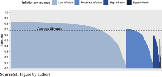
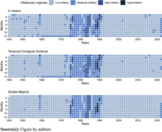
Figure 3 presents the classification over time of the estimated regimes, where each square represents a month, colored according to their associated inflationary regime. A significant portion of the observations belonging to the moderate, high, and hyperinflation regimes are concentrated between 1975 and 1991. The first is associated with the inflationary outbreak caused by the “Rodrigazo”, while the second corresponds to the disinflation resulting from the implementation of the Convertibility regime. These results are consistent with the evidence presented by Castagnino and D’Amato (2008) and D’Amato and Garegnani (2013) on the permanent impact on the inflationary dynamics of the “Rodrigazo”, which induced instability in the demand for money and the expectations of the agents. Also, an episode of high inflation can be identified at the beginning of 1959, a product of the crisis that occurred during the presidency of Arturo Frondizi. On the other hand, the latest data in the sample shows a transition of the Argentine economy to a moderate inflation regime in March 2022.
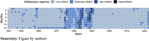
The figure displays the challenge of smoothing the classification explained in Section 3.2. It shows several months that have a regime change due to specific shocks to inflation. For instance, in the 1960s, December data are classified as a moderate inflation regime, despite the rest of the observations in the decade consistently falling under the low inflation regime.
Finally, based on the classification of regimes, we calculate a transition probability matrix, presented in Table 6. This matrix comes from the Markov Chains literature and describes the probability of transitioning from one regime to another in the following period. The low inflation regime is the most stable one, with a high probability that if the economy is in it, it will remain in it. On the other hand, if the economy is in hyperinflation, there is a probability of 60% that it will change state to a lower regime. These transition probabilities are not independent of the different macroeconomic policies that Argentina has implemented throughout its history.
4.2 Periodization
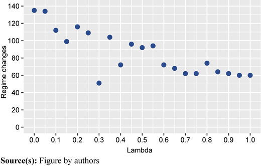
The value of λ used for the Temporal Contiguity Distance (TCD) is 0.1 [2], which expands the original distances by a maximum of 10%. In contrast, the Simple Majority (SM) periodization uses four lags corresponding to a voting window of five consecutive observations. Table 7 presents the results of the two smoothing techniques in comparison to the k-means estimation. Both methods achieve the desired outcome of reducing the number of regime changes, but the Simple Majority method achieves a greater reduction compared to the TCD method. Additionally, the table displays the total changes made compared to k-means, and it shows that the Simple Majority method makes the most replacements.
Comparison of classifications (k-means, TCD, SM)
| Regimes | k-means | TCD | SM |
|---|---|---|---|
| Low inflation | 738 | 724 | 771 |
| Moderate inflation | 175 | 183 | 144 |
| High inflation | 41 | 47 | 38 |
| Hyperinflation | 5 | 5 | 6 |
| Regime changes | 135 | 112 | 30 |
| Changes r/k-means | – | 58 | 92 |
Source(s): Table by authors
The regimes obtained by these methods preserve the results originally obtained by the ANOVA analysis. On the other hand, internal validation indices lose their usual interpretation when dissimilarity measures like TCD are used, as indicated by De Luca and Zuccolotto (2021).
Figure 4 presents the periodizations for the three methods. Consistent with the previous results, TCD produces a smoother classification, correcting the assignments of a group in the first decades of the sample and assigning the moderate inflation regime to points between 1979 and 1987. Nevertheless, it did not achieve the expected result in the months of December of the 1960s. On the other hand, the simple majority smoothing exhibited excellent performance in this regard, reducing the abrupt regime changes.
Temporal classification (k-means, TCD, SM)
Temporal classification (k-means, TCD, SM)
4.3 Discussion
To evaluate if the regimes proposed have a better performance than those of the literature, we perform a comparison exercise based on the analysis developed by Dabús (2000), later extended by Caraballo et al. (2006), for the inflation-relative prices relationship. Table 8 presents a comparison of the regimes for the entire sample, which are compared based on their order, which implies that the low inflation regime of this work will be taken as equivalent to the moderate inflation regime by Dabús (2000). The classification of this author differs significantly from the one developed in this paper, assigning more observations to moderate and high inflation regimes and fewer to the low inflation regime.
Regimes comparison
| Regimes | k-means | TCD | SM | Dabús |
|---|---|---|---|---|
| Low inflation (moderate) | 738 | 724 | 771 | 491 |
| Moderate inflation (high) | 175 | 183 | 144 | 376 |
| High inflation (very high) | 41 | 47 | 38 | 86 |
| Hyperinflation (idem) | 5 | 5 | 6 | 6 |
| Regime changes | 135 | 112 | 30 | 258 |
| Changes r/k-means | – | 58 | 92 | 294 |
Note(s): Classification of Dabús (2000) between brackets
Source(s): Table by authors
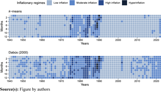
With almost twice as many regime changes as the k-means estimate, Figure 5 shows how the Dabús (2000) classification is much less smooth over time. Under this classification, in approximately a quarter of the sample, the regime at a given time differs from the regime of the previous period.
Temporal classification (k-means, Dabús)
Temporal classification (k-means, Dabús)
For this exercise, we use data from INDEC of the headline inflation and the inflation of the nine categories of the Consumer Price Index from September 1989 to December 2006 to assess the classifications for the inflation-relative price relationship. The regimes estimated previously with the full sample are used. Additionally, the following measure of relative price variability (RPV) is constructed based on Caraballo et al. (2006):
where wit is the weight of the category in the general index, πit is the inflation rate of the category i and πt is the headline inflation rate.
With these data, we estimate a linear model of relative price variability as a function of the monthly inflation rate. This model is used to assess the presence of structural changes for the inflationary regimes developed in this study (k-means, TCD, SM) and those presented by Dabús (2000). Table 9 presents the obtained estimates.
Inflation-relative price variability regressions
| Baseline | k-means | TCD | SM | Dabús | |
|---|---|---|---|---|---|
| RPV | RPV | RPV | RPV | RPV | |
| INF | 0.0069*** | 0.0076 | 0.0076 | 0.0140 | 0.0075 |
| (0.0007) | (0.0110) | (0.0124) | (0.0094) | (0.0206) | |
| MOD | 0.0007 | −0.0011 | 0.0010* | −0.0001 | |
| (0.0011) | (0.0008) | (0.0005) | (0.0007) | ||
| HIGH | 0.0006 | −0.0036** | 0.0045 | −0.0007 | |
| (0.0024) | (0.0013) | (0.0059) | (0.0009) | ||
| HYPER | 0.0033 | 0.0033 | 0.0097*** | 0.0094*** | |
| (0.0020) | (0.0020) | (0.0011) | (0.0016) | ||
| MOD∗INF | 0.0051 | 0.0294 | −0.0062 | 0.0044 | |
| (0.0152) | (0.0155) | (0.0096) | (0.0255) | ||
| HIGH∗INF | 0.0158 | 0.0245 | 0.0000 | 0.0213 | |
| (0.0123) | (0.0128) | (.) | (0.0210) | ||
| HYPER∗INF | −0.0055 | −0.0055 | −0.0154 | −0.0091 | |
| (0.0111) | (0.0125) | (0.0095) | (0.0206) | ||
| Constant | 0.0003* | 0.0001 | 0.0001 | 0.0000 | 0.0001 |
| (0.0001) | (0.0001) | (0.0001) | (0.0001) | (0.0001) | |
| Adjusted R2 | 0.297 | 0.595 | 0.608 | 0.561 | 0.558 |
| AIC | −2057.1 | −2167.0 | −2173.8 | −2150.8 | −2148.6 |
| BIC | −2050.4 | −2140.2 | −2147.0 | −2127.3 | −2121.9 |
| RMSE | 0.0018 | 0.0014 | 0.0013 | 0.0014 | 0.0014 |
| Observations | 210 | 210 | 210 | 210 | 210 |
| F (Chow) | – | 26.50 | 28.47 | 25.92 | 21.46 |
| p-valor | – | 0.000 | 0.000 | 0.000 | 0.000 |
Note(s): Standard deviations in parentheses
* **, *** indicate significance at 5, 1, and 0.1%, respectively
Source(s): Table by authors
For all classifications of regimes, we conclude in favor of the presence of breaks in the inflation-relative prices relationship, according to the results of the Chow (1960) test. Despite not being individually significant, the interaction terms are jointly significant for all classifications. These results suggest the presence of different relationships between inflation and relative prices in different inflationary regimes, which aligns with previous research.
In comparative terms, the three classifications presented show a better fit than the Dabús (2000) regimes [3]. Of the three, the simple majority procedure exhibits relatively the worst performance. A possible interpretation is that there is a trade-off between interpretability and explanatory capacity, i.e. the greater interpretability of the results is achieved at the cost of a loss of explanatory power due to the numerous changes made to the original classification.
The obtained classifications, which are country-specific, and the study of characteristics associated with the regimes provide a better understanding of the Argentine inflationary phenomenon. In addition, they could be used to identify factors related to transitions between regimes, which would serve as a “warning signal” for policymakers. In this sense, the classification could be used as complementary information, containing insights about the nature of each regime and the relation of them with other economic indicators.
However, we should be cautious when using these data and consider potential endogeneity issues when conducting econometric analyses. Furthermore, as with any monetary or price indicator, it is crucial to understand the feedback between the decisions made by the central bank and the classification itself since the central bank’s actions target the variable that is eventually classified. Nevertheless, if the classification is updated with each new data point, previous results should undergo marginal changes due to the structure of the data unless the incoming data points are outlier episodes, which could significantly alter the classification.
4.4 Illustration with Brazil and USA
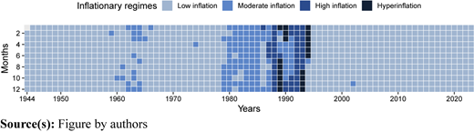
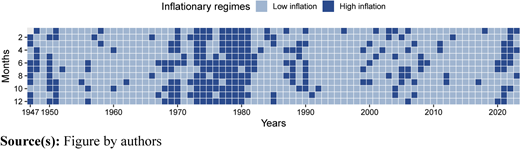
This subsection presents the results of applying the periodization method to other countries: Brazil and the USA. Brazil is included to demonstrate another Latin American country that experienced periods of high inflation throughout its history, while the United States serves as an example of a developed economy with historically more stable inflation. The data source for Brazil is the General Price Index-Domestic Supply (IGP-DI), retrieved from the Central Bank of Brazil. For the USA, we use the CPI for All Urban Consumers: All Items in U.S. City Average, from the FRED database. The results for Brazil are shown in Table 10 and Figure 6, while the results for the United States are presented in Table 11 and Figure 7.
Temporal classification Brazil (k-means, four regimes)
Temporal classification Brazil (k-means, four regimes)
Temporal classification United States (k-means, two regimes)
Temporal classification United States (k-means, two regimes)
Cluster-level descriptive statistics (Brazil)
| Regimes | Obs. | Average | SD | Thresholds | |
|---|---|---|---|---|---|
| Inflation | Min | Max | |||
| Low inflation | 770 | 1.28 | 1.27 | – | 4.96 |
| Moderate inflation | 125 | 8.62 | 3.02 | 4.96 | 16.32 |
| High inflation | 44 | 24.07 | 4.38 | 16.32 | 34.34 |
| Hyperinflation | 20 | 45.64 | 13.30 | 34.34 | – |
Note(s): The numbers correspond to monthly inflation rates
Source(s): Table by authors
Cluster-level descriptive statistics (United States)
| Regimes | Obs. | Average | SD | Thresholds | |
|---|---|---|---|---|---|
| Inflation | Min | Max | |||
| Low inflation | 668 | 0.13 | 0.21 | – | 0.42 |
| High inflation | 255 | 0.70 | 0.29 | 0.42 | – |
Note(s): The numbers correspond to monthly inflation rates
Source(s): Table by authors
As mentioned in the introduction, a crucial aspect of the methodology is selecting the number of regimes. Brazilian inflation with four regimes exhibits a behavior somewhat similar to that of Argentina, with a higher number of observations categorized as hyperinflation, though these have a lower average. While the threshold for Argentina was higher than the one of Cagan (1956), the one for Brazil is lower, with the economy transitioning to hyperinflation with a monthly rate higher than 30%. Despite having four regimes, Brazil’s instability is concentrated in the 1980s and early 1990s, showing low inflation for the remainder of the time series. This result contrasts with Argentina, which alternates between periods of low, moderate, and high inflation throughout the entire period.
In contrast, the USA, with two regimes, exhibits a very different history compared to Argentina (and Brazil). The 1970s and 1980s saw some periods of high inflation, but with averages significantly different from those of Latin American economies, with a mean of 0.30 for low inflation and 0.70 for high inflation. It is worth noting that with three clusters, the classification is unsatisfactory, as the periodization was not smooth but rather highly volatile. Although we refer to “high inflation” we are not implying that it is similar in characteristics to the high inflation regime identified in Argentina. In line with Dornbusch et al. (1990), “high inflation means different things to different people” (p. 2). In other words, what is considered high inflation varies between countries.
5. Conclusions
In this work, we sought to provide a classification of inflationary regimes that improved in methodological terms concerning the existing literature, appealing to a combination of machine learning techniques. The regimes obtained through these methods are specific to Argentine inflationary history and can be considered, in comparison with previous studies, as relatively free of bias from the researcher. Furthermore, these regimes are not formed through a forced grouping of the data and are independent of the relationships of interest on which one might later want to evaluate for the presence of breaks, unlike the threshold autoregressive models.
On the other hand, we introduce two procedures to achieve smooth periodizations over time. Both strategies effectively achieved a periodization with fewer regime changes over time, facilitating the interpretation and historical analysis of the results.
Finally, we determined that the classifications presented (k-means, TCD, and SM) provided a better explanatory power of the relationship between inflation and relative price variability than that of Dabús (2000). This highlights that, besides its methodological advantages, the proposed approach can provide a deeper understanding of inflation dynamics, which is crucial in developing more accurate forecasting models.
However, the methodological approach has certain limitations. Firstly, as mentioned in the methodology section, clustering techniques are known for their great sensitivity to the data employed, which makes the results very unstable to alterations in the sample used. Additionally, the specific nature of the subject meant that objective criteria could not be used to select the number of regimes. On the other hand, the limited availability of data and the manipulation of official inflation statistics led to the fact that only the monthly inflation rate could be used as an input without being able to capture other relevant aspects of the regimes.
Based on the results obtained, future lines of research could be followed to improve and expand the proposed methodology. One of the areas of interest would be to extend the application to a larger sample of countries, to compare the regimes obtained between them, extending the work conducted in Section 4.4. On the other hand, it is necessary to develop a temporal clustering technique, which allows smoothing of the classification over time, regardless of the measure used.
We thank Fernando Tohmé and conference participants of the L Argentine Statistics Colloquium for their valuable comments and suggestions.
Funding: This research was funded by PGI UNS 24-E172 granted to Fernando Delbianco and CIN 452/22 granted to Manuel de Mier.
Notes
Strictly, the TCD constitutes a measure of dissimilarity, since it meets the conditions of non-negativity, identity, and symmetry, but not that of triangular inequality. Nevertheless, none of these properties are essential to perform a cluster analysis (Kaufman & Rousseeuw, 2009).
The choice of lambda is supported by Figure A4 in Appendix 1, which illustrates the regime changes for various lambda values (at steps of 0.05). As anticipated, an inverse relation between regime changes and lambda values is demonstrated, albeit in a non-monotonic manner. This non-uniform trend may be attributed to the intermediate step of the principal coordinate analysis employed. The graph indicates a noteworthy initial decline in regime changes at a value of 0.1.
Since this is a goodness-of-fit exercise, the results are invariant to the consideration of heteroskedasticity or autocorrelation since they do not depend on the standard errors of the coefficients.
References
Appendix 1 Optimal number of clusters
This appendix shows the traditional methods for selecting the optimal number of clusters: the elbow method (Figure A1), the average silhouette method (Figure A2), and the gap statistic method (Figure A3). Additionally, Figure A4 illustrates the inverse but non-monotonic relationship between lambda values and regime changes, highlighting a notable decline at a lambda value of 0.1.
Regime changes for varying lambda
Regime changes for varying lambda
Appendix 2 Robustness analysis for different number of regimes
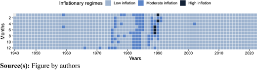
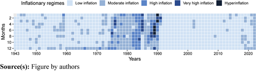
This appendix details the results of inflation clustering for Argentina using three and five regimes. For the three regimes, results are shown in Table A1 and Figure A5, while Table A2 compares the classification with the four-regime classification. Similarly, results for the five regimes are presented in Table A3 and Figure A6, with Table A4 providing a comparison with the four-regime classification. In the first case, only hyperinflation remains as high inflation, forcing a lot of variability in moderate inflation. In the second case, the breakdown between high and very high inflation is forced and with few representative data for the very high case.
Cluster-level descriptive statistics (three regimes)
| Regimes | Obs. | Average | SD | Thresholds | |
|---|---|---|---|---|---|
| Inflation | Min | Max | |||
| Low inflation | 868 | 2.25 | 2.69 | – | 10.17 |
| Moderate inflation | 86 | 18.15 | 8.61 | 10.17 | 70.02 |
| High inflation | 5 | 112.86 | 49.08 | 70.02 | – |
Note(s): The numbers correspond to monthly inflation rates
Source(s): Table by authors
Comparison of the classification between three and four clusters
| Low inflation | Moderate inflation | High inflation | |
|---|---|---|---|
| Low inflation | 738 | 0 | 0 |
| Moderate inflation | 130 | 45 | 0 |
| High inflation | 0 | 41 | 0 |
| Hyperinflation | 0 | 0 | 5 |
Source(s): Table by authors
Cluster-level descriptive statistics (five regimes)
| Regimes | Obs. | Average | SD | Thresholds | |
|---|---|---|---|---|---|
| Inflation | Min | Max | |||
| Low inflation | 659 | 1.01 | 1.43 | – | 3.67 |
| Moderate inflation | 219 | 6.36 | 2.01 | 3.67 | 10.93 |
| High inflation | 60 | 15.54 | 3.33 | 10.93 | 23.97 |
| Very high inflation | 16 | 9.12 | 8.92 | 23.97 | 70.02 |
| Hyperinflation | 5 | 112.86 | 49.08 | 70.02 | – |
Note(s): The numbers correspond to monthly inflation rates
Source(s): Table by authors
Comparison of the classification between five and four clusters
| Low inf. | Moderate inf. | High inf. | Very high inf. | Hyperinflation | |
|---|---|---|---|---|---|
| Low inflation | 659 | 79 | 0 | 0 | 0 |
| Moderate inflation | 0 | 140 | 35 | 0 | 0 |
| High inflation | 0 | 0 | 25 | 16 | 0 |
| Hyperinflation | 0 | 0 | 0 | 0 | 5 |
Source(s): Table by authors
Temporal classification (k-means, three regimes)
Temporal classification (k-means, three regimes)
Temporal classification (k-means, five regimes)
Temporal classification (k-means, five regimes)

