


The paper examines the impact of COVID-19 on bank stock returns over various time scales and frequencies for 36 countries. Moreover, the authors look at the governments' responses to the corona crisis and examine its impact on bank stock returns.
The paper applies continuous wavelet transformation to obtain robust estimates of the co-movement (coherency) between confirmed cases and bank stock returns over time and at different time scales. Furthermore, the authors apply fixed effects panel regression to examine the response of bank stocks to domestic COVID-19 policies.
The results indicate that the number of confirmed COVID-19 cases negatively impacts bank stock returns during different waves of the pandemic in the medium-run. However, there is only little dependence in the very short-run. Moreover, bank stock returns positively react to domestic COVID-19 polices. This demonstrates that governmental interventions not only reduce the spread of COVID-19 but are also able to thereby calm financial markets.
The application of wavelet methods to the field of economics and finance is relatively recent and allows the distinction between short-term and long-term effects. Standard econometric methods, in contrast, only operate within the time domain. This paper combines wavelet methods with conventional econometrics to answer the research question.
1. Introduction
The ongoing corona crisis has been affecting the international financial markets for almost two years. A continuously growing body of research demonstrates that the COVID-19 pandemic increases the systematic default risk in the eurozone (Ito, 2020), adversely affects crude oil prices, and raises stock market volatility all over the world (Jeris & Nath, 2021). In addition, the studies of Topcu and Gulal (2020), Al-Awadhi, Alsaifi, Al-Awadhi, and Alhammadi (2020), He, Sun, Zhang, and Li (2020), and Mazur, Dang, and Vega (2021) demonstrate a negative impact on stock returns, with a varied magnitude across branches. While food, healthcare, and software stocks are less impacted by the pandemic, transportation, electricity, and environment stock returns decreased sharply. Miescu and Rossi (2021) show that COVID-19-induced shocks hit most harshly the industries relying on face-to-face interactions. Moreover, Acharya, Engle, and Steffen (2021) and Dunbar (2021) show a significant underperformance of bank stock returns relative to other firms, which they attribute to high degrees of the balance-sheet liquidity risk. Accordingly, Duan, Ghoul, Guedhami, Li, and Li (2021) show that the COVID-19 pandemic increases the systemic risk in the banking sector, where the adverse effects are more pronounced for large and highly leveraged banks. In addition, some studies show that bank lending is significantly lower in the countries that are more affected by the pandemic, while the response of the public health sector to the crisis has a positive effect on bank lending (Çolak and Özde Öztekin, 2021). Demirgüç-Kunt, Pedraza, and Ruiz-Ortega (2021) specifically demonstrate that financial sector policy announcements, such as liquidity support, borrower assistance programs and monetary easing reduce the adverse impact of the pandemic on bank stocks. Finally, Yousfi, Zaied, Cheikh, Lahouel, and Bouzgarrou (2021) compute dynamic conditional correlations in order to assess and compare the impacts of the first and second pandemic waves in the United States and reveal a persistent link between returns, uncertainty, and the COVID-19 pandemic during both waves of the outbreak.
As banks are important for the financial stability in a country, the present study also focuses on the banking sector but contributes to the fast-growing research with two main points. First, we apply wavelet transformation to capture the waving pattern in the number of confirmed COVID-19 cases and obtain robust estimates of the co-movement between confirmed cases and bank stock returns over time and at different time scales. These time-scale effects and thus knowledge about short-run and long-run impacts, are of a considerable importance for policymakers and investors. Second, we look at the governments' responses to the corona crisis and examine their possible impacts on bank returns by employing fixed effect panel regression with interaction effects. Prior research focuses on the impact of COVID-19 policy regulations on other sectors such as energy commodities (Czech & Wielechowski, 2021), travel, tourism, leisure stock market (Wang, Zhang, Gao, & Yang, 2021; Yang, Mao, & Wen, 2021), and local food prices (Dietrich, Giuffrida, Martorano, & Schmerzeck, 2022) rather than banks.
2. Data and methodology
The analysis is based on the daily Financial Times Stock Exchange (FTSE) bank stock market indices for a period from January 01, 2020, to June 01, 2021. The indices comprise a series of large and medium-sized banks in country j. Due to non-stationarity, bank stock returns are computed as the first difference of the natural log in line with . Non-trading weekends are excluded from the data sample. The daily number of confirmed COVID-19 cases per one million people for each country is collected from the World Health Organization (WHO). Overall, the sample comprises 36 countries, which are listed in Table 1.
The countries included in the sample
| AU | Australia | FR | France | JP | Japan | ZA | South Africa |
| AT | Austria | DE | Germany | MY | Malaysia | KR | South Korea |
| BE | Belgium | GR | Greece | MX | Mexico | ES | Spain |
| BR | Brazil | HU | Hungary | NO | Norway | SW | Sweden |
| CA | Canada | IN | India | PL | Poland | CH | Switzerland |
| CO | Colombia | ID | Indonesia | QA | Qatar | TW | Taiwan |
| CZ | Czech Republic | IE | Ireland | RO | Romania | TH | Thailand |
| DK | Denmark | IL | Israel | RU | Russia | UK | United Kingdom |
| EG | Egypt | IT | Italy | SG | Singapore | US | United States |
2.1 Univariate wavelet transform
Wavelet transformation decomposes a time series xt into a set of daughter functions, which are derived from a mother wavelet through scaling and translation in time. Hence, the mother wavelet can be expressed as a function of the translation parameter τ and the scale parameter s. While the latter defines how the wavelet is stretched, the translation parameter determines the position of the wavelet. The general shape is given by
where the normalization factor ensures comparability across different time series and scales (Vacha & Barunik, 2012; Tiwari, Mutascu, & Albulescu, 2016). Moreover, ⋆ denotes the complex conjugate and t indicates the time component. Based on the number of different mother wavelets, the Morlet function introduced by Grossmann and Morlet (1984) is utilized
The Morlet wavelet is the most common specification in the field of economics and finance, as it secures the best trade-off between time and frequency localization (Singh, Das, Jana, & Tiwari, 2018; Wu & Wu, 2019; Stolbov, Karminsky, & Shchepeleva, 2018). Moreover, the Morlet is a complex wavelet, wherefore the continuous wavelet transform can be divided into real and imaginary denoted by i. The angular frequency parameter of Equation (2) is set to ω = 6, which inversely links the wavelet scale to the frequency. The relation is used to convert the frequency into days to ease the economic interpretations within this study.
2.2 Cross-wavelet transform
The cross-wavelet analysis assesses the co-movement of two time series with respect to their periodic components and development over time (Schmidbauer, Rösch, & Uluceviz, 2017). The cross-wavelet transform of two time series xt and yt is presented by
where the complex wavelet coherency is defined as
provided that S denotes a smoothing operator in time and scale. Finally, the absolute value of Γxy(τ, s) depicts the wavelet coherency denoted as
The coherency measures the local correlation between xt and yt in the time-frequency space with 0 ≤ Rxy(τ, s) ≤ 1. Values close to 1 show a high correlation, where the dependence can be negative or positive. The time-frequency relations are usually visualized with heat maps. The significance is assessed by testing the dependency patterns against simulated white noise (Ko & Funashima, 2019; Bales, 2022). In the specific case, the null hypothesis of white noise states that there are no significant interrelations over time and that there is no periodicity between daily new COVID-19 cases and FTSE bank returns in a country.
2.3 Cross-wavelet phase angle
Due to its complex feature, the cross-wavelet transform carries information about the synchronicity of two time series in terms of the local phase. The resulting Anglexy(τ, s) is the phase difference of xt over yt at each scale and time computed as
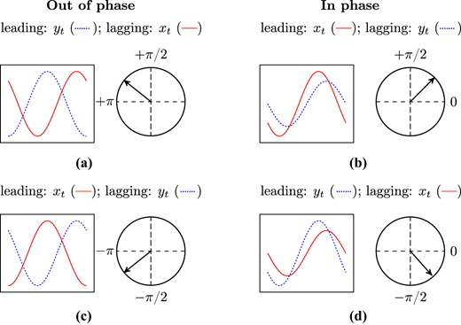
where Phasex(τ, s) and Phasey(τ, s) are angles in the interval [− π; + π]. Both measure the displacement of a periodic component relative to an origin in the time domain (Schmidbauer et al., 2017; Bales, 2022). An absolute value less (higher) than π/2 indicates that the two time series move in-phase (anti-phase), stating that both change in the same (different) direction (Stolbov et al., 2018; Schmidbauer et al., 2017). The lead-lag patterns can be illustrated with arrows in cross-wavelet heat maps. Figure 1 depicts the interpretation of these arrows. The time series in Panel (b) and Panel (d) move in-phase, while the series in Panel (a) and Panel (c) move anti-phase.
3. Results and discussion
Figures 2–4 visualize the wavelet coherency between FTSE bank returns (xt) and daily new COVID-19 cases (yt) for each country. The vertical axis corresponds to the wavelet scale expressed in business days; The horizontal axis captures the time domain from January 01, 2020, to June 01, 2021. The red and orange colors indicate regions of high dependence between bank returns and new cases, while the blue and turquois colors are associated with no or little dependence. The black contour lines depict the time-period domain of joint significance at the level of 1%. The arrows pointing left-up show that both series move in opposite directions, where the number of daily COVID-19 cases leads banking sector returns. Conversely, the arrows pointing left-down show that bank returns (inversely) lead the number of new cases. Arrows pointing to the right indicate a positive relationship between both series, implying that the stock markets do not fear greater infection rates.
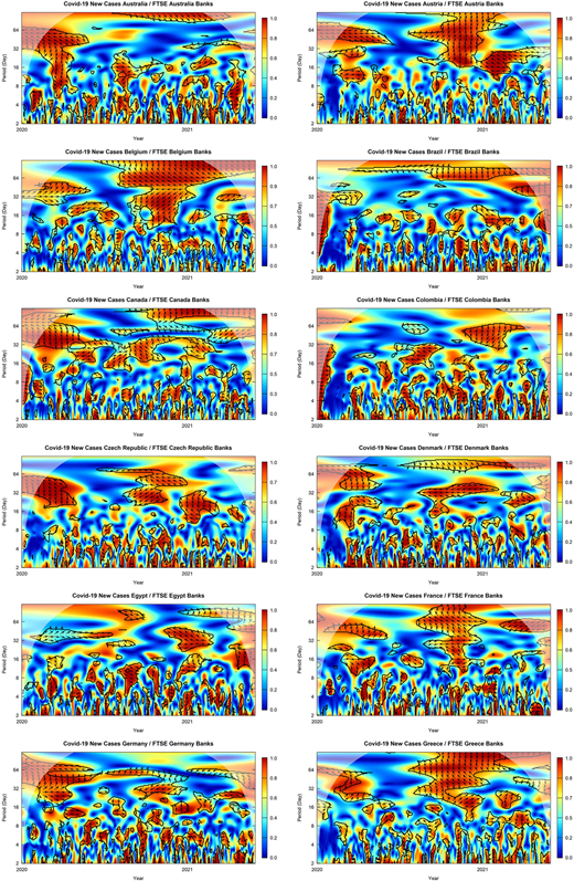
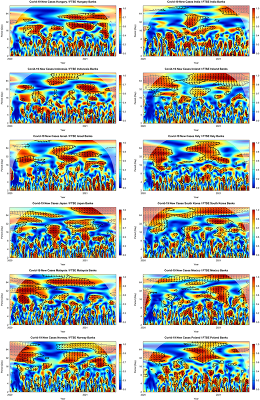
Wavelet coherency between new confirmed COVID-19 cases and bank stock returns II
Wavelet coherency between new confirmed COVID-19 cases and bank stock returns II
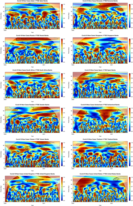
Wavelet coherency between new confirmed COVID-19 cases and bank stock returns III
Wavelet coherency between new confirmed COVID-19 cases and bank stock returns III
Considering the wavelet coherency patterns in Figures 2–4, almost all of the countries exhibit two areas of high dependence. Apart from the initial crash of the stock markets between February and April 2020, a second area of high (negative) co-movement ranges from the last quarter of 2020 until mid-2021. During the first wave, arrows pointing left-up indicate that the number of confirmed COVID-19 cases leads banking sector stock returns. Thus, increased infection rates and related market fear had a significant negative impact on bank stock returns. These co-movements are mainly observable for the frequency bands between 16 and 72 days, showing that the pandemic primarily affects bank returns in the medium-run. In contrast, there is only little dependence in the very short-run (period <8 days). Overall, the coherency is stronger in European countries and the United States, which underpins the study of Acharya et al. (2021).
In some countries, the financial markets exhibit a stronger response to the second wave rather than the initial shock. Exemplarily, Austria, Belgium, France, Greece, Poland, Switzerland, and Sweden show a high (negative) correlation between new cases and bank returns during that period, where the causality is mainly from the former to the latter. During the summer of 2020, low infection rates triggered positive expectations that the pandemic could be under control soon. However, sharply rising infections at the end of the year brought back the concerns and the financial markets reacted with fear. While Sweden was initially known for its “alternative” way to handle the pandemic with fewer restrictions compared to other European states, the second wave hit Sweden and its financial markets relatively hard. Looking at the most recent developments, the financial markets in Brazil and India are affected by sharply increasing infection rates. The opposite is observed for the US and Australia. Driven by low cases and high vaccination rates, the markets are optimistic and less exposed to the COVID-19 fear during the second wave.
The possible way of impact can be explained as follows. Considering a basic model with a production and financial sector, households lend money to banks. Banks, in turn, provide credits to firms, which use these loans to make investments. Increasing uncertainty about the COVID-19 virus and threatening economic risks of the pandemic has led households to reduce consumption and increase precautionary savings. At the same time, firm investments and credit demand are expected to decrease due to a wait-and-hold strategy, which consequently affects bank revenues. As uncertainty generally bears risk, banks tend to further tighten their lending activity by rigorously monitoring their borrowers, which further cuts down profits (Swamy, 2013). In this context, Bordo, Duca, and Koch (2016) indicate a significant negative relation between uncertainty and bank credit growth in the United States. Furthermore, governmental lock-down policies and sales shortfalls increase the overall default risk of firms in an economy. Finally, the threatening payment defaults of creditors affect bank profits and the stock price. As global banks are highly connected, the effects are further amplified by cross-country risk spillovers and contagion. Foglia, Addi, and Angelini (2021) reveal that global banks are highly interconnected in terms of volatility, reaching their 15-year maximum peak at the time of COVID-19. Moreover, the authors argue that the Eurozone banking system is too “interconnected to fail” because of heavy risk spillovers affecting banking stability.
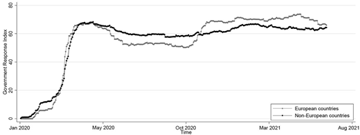
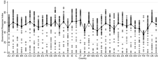
In a complementary analysis, the impact of the governments' COVID-19 policies on the banking sector is assessed. The overall response in each country is measured by the Oxford COVID-19 government response tracker (GR) from the Blavatnik School of Government at the University of Oxford (Hale et al., 2021). The daily index consists of several categories, such as closure policies (school, workplace), testing and vaccination strategies, and economic support. The index ranges from 0 to 100, where higher values illustrate a stricter response of the government. In particular, this could be a stricter closing policy, a greater amount of economic support for companies, or higher vaccination rates. Figure 5 shows the development of the government response tracker over time. After the first wave, European [1] countries relaxed their COVID-19 policy and restrictions quicker than other states. In the course of the pandemic, however, the European countries have tightened the restrictions again strongly, ending up with greater limitations than in many non-European countries. Moreover, Figure A1, highlights the heterogeneity in governments' responses across countries.
Econometrically, governments' impacts on bank returns are estimated by a fixed effects panel regression model specified as
where represents bank stock returns for country j at time t computed as the first difference of the natural log of the FTSE banking sector indices. Moreover, αj and λt capture the country and time fixed effects, respectively, and j,t is a zero-mean random error term. Casesj,t measures the change in new COVID-19 cases per million people in country j at time t and DEMV captures the daily infectious disease equity market volatility tracker of Baker et al. (2020)[2]. In the course of this study, the DEMV index is considered as an alternative measure of global COVID-19 fear, and to assess the robustness of the results. Finally, the interaction term between the governmental response and the number of new cases is included. The model is estimated in different specifications, with standard errors clustered at the country level. The regression results are depicted in Table 2.
Panel regression results
| (1) | (2) | (3) | (4) | (5) | (6) | |
|---|---|---|---|---|---|---|
| b/se | b/se | b/se | b/se | b/se | b/se | |
| Cases | −0.7632∗∗∗ (0.2793) | −0.7586∗∗∗ (0.2764) | −0.9853∗∗∗ (0.3614) | −0.8092∗∗∗ (0.2661) | −0.8092∗∗∗ (0.2661) | |
| GR | 0.0062∗∗ (0.0028) | 0.0124∗∗∗ (0.0011) | 0.0060∗∗ (0.0028) | 0.0060∗∗ (0.0028) | 0.0105∗ (0.0052) | |
| Cases × GR | 0.0030∗∗ (0.0011) | 0.0016∗∗ (0.0006) | 0.0016∗∗ (0.0006) | |||
| DEMV | −0.4809∗∗∗ (0.1055) | −0.1651∗∗ (0.0632) | ||||
| DEMV × GR | −0.0002 (0.0002) | |||||
| Constant | 1.2075∗∗∗ (0.2516) | 1.2039∗∗∗ (0.2525) | −0.6948∗∗∗ (0.0607) | 1.2040∗∗∗ (0.2527) | 2.5698∗∗∗ (0.5269) | 0.3098∗∗ (0.1212) |
| Time-FE | Yes | Yes | No | Yes | Yes | Yes |
| Country-FE | Yes | Yes | Yes | Yes | Yes | Yes |
| Obs | 13248 | 13248 | 13248 | 13248 | 13248 | 13284 |
| No. of countries | 36 | 36 | 36 | 36 | 36 | 36 |
| R2 | 0.41 | 0.42 | 0.18 | 0.42 | 0.43 | 0.42 |
Note(s): The standard errors are clustered at the country level. ∗p < 0.10, ∗∗p < 0.05, ∗∗∗p < 0.01
In line with the prior results, Table 2 indicates a significant negative COVID-19 impact on bank stock returns. Furthermore, the regression results reveal a positive influence of the COVID-19 government response tracker in Model 2. In addition, the interaction between both variables is of importance. This demonstrates that governmental interventions not only reduce the spread of COVID-19 but also mitigate the negative impact on bank stocks as
By increasing GRj,t, governments can offset some of the adverse effects as β3 > 0. Finally, Model 5 and Model 6 show a negative impact of infectious disease equity market volatility on bank returns, while the interaction term is not significant. The latter can be explained by the fact that a government most likely responds to the number of domestic cases rather than the unobserved global volatility. The results are robust against (1) the inclusion of domestic bank CDS premia to control the overall bank default risk (2) the MSCI World stock market index in order to capture the worldwide stock market dynamics (3) the VIX and VSTOXX volatility indices to take general macroeconomic uncertainty into account and (4) domestic economic policy uncertainty to differentiate between general economic policy uncertainty and COVID-19 related governmental policies (Table A1). Overall, the findings continue prior research of Narayan, Phan, and Liu (2021) and Chang, Feng, and Zheng (2021), extending its applicability to a much greater number of countries and a more updated time period.
Robustness checks
| (1) | (2) | (3) | (4) | (5) | (6) | |
|---|---|---|---|---|---|---|
| b/se | b/se | b/se | b/se | b/se | b/se | |
| Cases | −0.8323∗∗ (0.3667) | −0.8250∗∗ (0.3656) | −0.9336∗∗ (0.3547) | −0.9325∗∗ (0.3540) | −0.9423∗∗∗ (0.3432) | |
| Bank CDS | −0.0595∗∗∗ (0.0079) | −0.0585∗∗∗ (0.0079) | −0.0585∗∗∗ (0.0079) | −0.0585∗∗∗ (0.0079) | −0.0556∗∗∗ (0.0079) | −0.0547∗∗∗ (0.0080) |
| EPU | −0.0021∗∗∗ (0.0004) | −0.0020∗∗∗ (0.0003) | −0.0020∗∗∗ (0.0003) | −0.0020∗∗∗ (0.0003) | −0.0015∗∗∗ (0.0003) | −0.0015∗∗∗ (0.0003) |
| MSCI World | 0.7618∗∗∗ (0.0613) | 0.7594∗∗∗ (0.0612) | 0.7538∗∗∗ (0.0606) | 0.7594∗∗∗ (0.0612) | 0.7553∗∗∗ (0.0612) | 0.7530∗∗∗ (0.0615) |
| VIX | 0.0358∗∗∗ (0.0031) | 0.0364∗∗∗ (0.0031) | 0.0364∗∗∗ (0.0031) | 0.0364∗∗∗ (0.0031) | 0.0365∗∗∗ (0.0031) | 0.0364∗∗∗ (0.0031) |
| VSTOXX | −0.0408∗∗∗ (0.0080) | −0.0403∗∗∗ (0.0079) | −0.0413∗∗∗ (0.0083) | −0.0403∗∗∗ (0.0079) | −0.0414∗∗∗ (0.0079) | −0.0410∗∗∗ (0.0078) |
| GR | 0.0048∗∗∗ (0.0009) | 0.0045∗∗∗ (0.0009) | 0.0044∗∗∗ (0.0010) | 0.0062∗∗∗ (0.0011) | 0.0048∗∗∗ (0.0014) | |
| Cases × GR | 0.0033∗∗∗ (0.0010) | 0.0034∗∗∗ (0.0010) | 0.0024∗∗ (0.0009) | |||
| DEMV | −0.0112∗∗∗ (0.0018) | −0.0179∗∗∗ (0.0042) | ||||
| DEMV × GR | 0.0001 (0.0001) | |||||
| Constant | −0.0513∗∗∗ (0.0040) | −0.3118∗∗∗ (0.0498) | −0.3136∗∗∗ (0.0492) | −0.3077∗∗∗ (0.0512) | −0.1914∗∗∗ (0.0447) | −0.1293∗∗ (0.0518) |
| Time-FE | Yes | Yes | No | Yes | Yes | Yes |
| Country-FE | Yes | Yes | Yes | Yes | Yes | Yes |
| Obs | 13248 | 13248 | 13248 | 13248 | 13248 | 13284 |
| No. of countries | 36 | 36 | 36 | 36 | 36 | 36 |
| R2 | 0.58 | 0.58 | 0.34 | 0.61 | 0.62 | 0.58 |
Note(s): Robust standard errors are lustered at the country level. ∗p < 0.10, ∗∗p < 0.05, ∗∗∗p < 0.01
4. Conclusion
This study applies wavelet coherency analysis to examine the impact of new COVID-19 cases on bank stock returns for 36 countries. The results show that the number of new infections and related fear has a significant negative impact on bank returns during different waves of the pandemic for the frequencies between 16 and 72 days. In contrast, there is only little dependence in the very short-run. Moreover, this paper shows that a more powerful governmental response in the form of workplace and school closures, greater economic support, or a stricter testing policy has a positive impact on bank stock returns. Hence, governmental interventions not only reduce the spread of COVID-19 but are also able to calm the financial markets. These findings provide important implications for policymakers, regulatory bodies and investors related to the background of the ongoing pandemic.
Notes
European countries: AT, BE, CZ, DK, FR, DE, GR, HU, IE, IT, NO, PL, RO, ES, SW, CH, UK.
All variables are concluded to be stationary, resulting from Augmented Dickey Fuller tests.
This work was supported by the German Academic Scholarship Foundation.

