
The purpose of this study is to investigate the transport phenomena of smoke flow in a semi-open vertical shaft.
The large eddy simulation (LES) method was used to model the movement of fire-induced thermal flow in a full-scale vertical shaft. With this model, different fire locations and heat release rates (HRRs) were considered simultaneously.
It was determined that the burning intensity of the fire is enhanced when the fire attaches to the sidewall, resulting in a larger continuous flame region in the compartment and higher temperatures of the spill plume in the shaft compared to a center fire. In the initial stage of the fire with a small HRR, the buoyancy-driven spill plumes incline toward the side of the shaft opposite the window. Meanwhile, the thermal plumes are also directed away from the center of the shaft by the entrained airflow, but the inclination diminishes as HRR increases. This is because a greater HRR produces higher temperatures, resulting in a stronger buoyancy to drive smoke movement evenly in the shaft. In addition, a dimensionless equation was proposed to predict the rise-time of the smoke plume front in the shaft.
The results need to be verified with experiments.
The results could be applied for design and assessment of semi-open shafts.
This study shows the transport phenomena of smoke flow in a vertical shaft with one open side.
1. Introduction
High-rise building fires have attracted increasing attention from researchers in recent times, especially after some major accidents (Hall, 2013). High-rise buildings are those that are taller than 23 m according to the classification of the National Fire Protection Association (NFPA) (Cote, 2012). In reality, smoke laden with toxic gases produced by fires is the most deadly threat to the life and safety of residents, and statistical analyses have shown that approximately 85 per cent of deaths were caused by toxic smoke (Alarie, 2002). In modern high-rise buildings, there are numerous shaft-like spaces, which can have many forms, including stairwells, electric cable shafts, elevator shafts and dumbwaiter shafts. In addition, to meet functional requirements, a large number of shafts with open ceilings are embedded in buildings to provide natural ventilation and light, with the aim of conserving energy and improving occupant comfort.
Based on these different functions, vertical shafts can be roughly classified into two types: those with and without ceilings. During building fires, fire development may be worsened by shaft-like structures because they encourage the thermal smoke to move upwards. In general, the vertical transport of fire-induced smoke flow is mainly driven by two mechanisms: turbulent mixing and the stack effect (Zukoski, 1995), which correspond to shafts with and without ceilings, respectively. Meanwhile, it should be noted that a precondition for these relationships in the current study is that all doors and windows connected to the shaft are closed.
The turbulent mixing is commonly referred to as the Rayleigh–Taylor instability, which occurs when a light fluid lies below a heavy fluid in a gravitational field (Taylor, 1950; Andrews and Spalding, 1990). This results in the mixing of two fluids with different densities in the presence of gravitational instability. When there is no stack effect during a building fire, the transport of fire-induced smoke flow is primarily driven by turbulent mixing through the compartment to the vertical shaft. Many previous experiments have investigated the characteristics of the instability movement of two fluids driven by turbulent mixing (Taylor, 1950; Cannon and Zukoski, 1975; Cannon, 1976; Andrews and Spalding, 1990; Snider and Andrews, 1994; Ji et al., 2015a; Ji et al., 2015c), including one-dimensional mixing phenomena (Andrews and Spalding, 1990), the combined effects of shear and buoyancy (Snider and Andrews, 1994) and the effect of the location of openings in stairwells on the transport of thermal smoke induced by fires (Ji et al., 2015a; Ji et al., 2015c). Turbulent mixing typically occurs in shafts with ceilings, such as stairwells without upper openings.
In contrast, when building fires occur in a compartment connected to a shaft without a ceiling, the transport of thermal smoke can be primarily driven by the stack effect, which is caused by the temperature-induced air pressure and density differences between the interior and exterior of a shaft or between two interior spaces (Strege and Ferreira, 2017). If the stack effect is a major driving force of smoke movement in a building fire, then fire-induced thermal flow carrying high-temperature toxic gas could be induced to move upwards rapidly. Therefore, it is expected that the hazards because of the stack effect are greater than those from turbulent mixing. To understand the transport characteristics of thermal smoke driven by the stack effect in shafts, many studies have been carried out through both experiments (Hiroomi et al., 1994; Benedict, 1999; Su et al., 2011; Shi et al., 2014) and simulations (Xiao et al., 2008; Sun et al., 2011; Harish and Venkatasubbaiah, 2013; Chen et al., 2016). However, the sidewalls of the vertical shaft have commonly been assumed to be sealed in previous studies, with only a single opening near the ceiling. In reality, a kind of semi-open vertical shaft has been widely applied in high-rise buildings in China to supply natural ventilation and light (Li et al., 2015). In this type of semi-open vertical shaft, the side connected to the corridor is open, while the other three sides of the shaft are sealed by solid walls. At present, there are less studies focused on the transport characteristics of fire-induced thermal smoke in a shaft (Li et al., 2015), and some basic data including the vertical temperature distribution and smoke spread velocity were not measured, and the flow field was not also presented.
In this study, a numerical method was used to simulate fire-induced smoke movement through a compartment connected to a semi-open vertical shaft in a full-scale high-rise building. The aim was to investigate the transport phenomena of smoke, including the vertical temperature distribution and flow field in the shaft. During the simulations, varying heat release rates (HRRs) of the fire source were considered. In addition, two different fire locations in the compartment were considered because fire can occur at any location as a result of an electrical short circuit or other causes.
2. Simulation setup
2.1 Introduction to FDS
The Fire Dynamics Simulator (FDS) is a computational fluid dynamics (CFD) model developed by the National Institute of Standards and Technology (NIST) to simulate fire-induced environments (McGrattan et al., 2015). It includes two models: direct numerical simulation (DNS) and large eddy simulation (LES). The LES model is used in this study owing to its wide application in the field of buoyancy-driven thermal flow movement. To calculate a fire scenario, users must first build a physical model and then divide it into a large number of grids with a fixed size, which serve as the basic unit of the numerical simulation. The modeling is then worked in each grid to solve a set of viscous fluid equations, that is, the Navier–Stokes equations. Finally, typical fire parameters such as temperature, velocity, gas concentration and visibility in a plane can be monitored and output during simulations. In addition, the distribution of temperature, pressure and velocity can be observed in any desired plane. As FDS is gradually improved, its reliability and practicability have been repeatedly verified for shaft fire scenarios (Chen et al., 2015; Li et al., 2018).
2.2 Physical model and fire scenarios
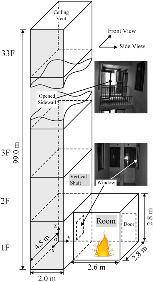
In this study, a full-scale vertical shaft model was used, as described in a previous publication (Li et al., 2015). Figure 1 shows the schematic of the building structure, which is a 33-story high-rise building with a height of 99 m, and includes a shaft and a compartment that is designed as a bedroom. Each floor is 2.8 m high and has a 0.2 m thick floor slab. The cross-sectional dimensions of the shaft and compartment are 4.5 m × 2 m and 2.8 m × 2.6 m, respectively. As Figure 1 shows, the front side and ceiling of the shaft are open, and thus, their boundaries are set as “OPEN.” To allow the fire-induced smoke to flow freely, an open window with 1 m wide and 1.5 m high connects the shaft and compartment. However, the compartment door is always closed. In addition, the lining material of the building construction is specified as “CONCRETE,” and its density, specific heat and conductivity are 2200 kg/m3, 0.88 kJ/(kg K) and 1.2 W/(m K), respectively (Ji et al., 2015b). The ambient temperature is 20°C.
Sectional views of the shaft model are shown in Figure 2. As Figure 2(a) shows, a pool fire with a size of 1 × 1 × 0.5 m is set in the compartment. Although the sidewall effect has been widely studied under confined ceilings, such as in tunnel fires (Zhou et al., 2017), it has not been reported in enclosure fires. Therefore, two different fire locations are considered. The transverse distances between the fire centers and the window are 1.3 m and 2.1 m, which correspond to a center fire and a wall fire, respectively. In this study, four pool fires with different HRRs are modeled, that is, 0.5 MW, 1 MW, 2 MW and 3 MW, which can be used to simulate different fire stages, from the initial stage to the flashover stage. In the simulations, 33 thermocouples are located in the shaft to monitor the temperature variations in real time. Except for TC 1, which is located between floors 1 and 2, all of the thermocouples are fixed at the center of each floor.
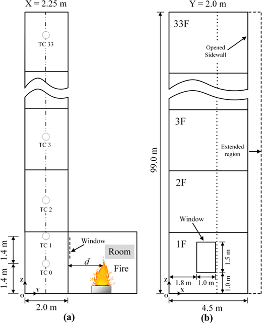
According to the FDS user guide (McGrattan et al., 2015), the ratio is used to evaluate the grid resolution, and its recommended value is within the range of 4-16. This means that the required cell size, δx, decreases with the reduction of the heat release rate, Q. For a 0.5 MW fire, the grid size should be 0.04-0.18 m. In consideration of the limits of computing resources, a uniform multi-grid system was used in this study. Hence, a grid cell size of 0.1 m was employed in the shaft, while a finer cell size of 0.05 m was used for the compartment area. As Figure 2(b) shows, reasonable extension of the domain in the direction of the x-axis was also confirmed to produce accurate results. Based on the original scale of 4.5 m, the computational domain is extended by 1.5 m and 3 m. The results show that extension of the domain has a significant impact on the temperature field. An extension size of 1.5 m was selected, and its temperature error was approximately 7 per cent compared to the larger domain of 3 m.
3. Results and discussion
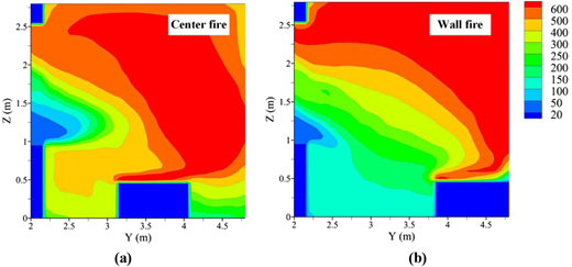
During the simulations, two different fire locations were considered, that is, a center fire and a wall fire. Temperature contours at the x = 2.25 m plane in the compartment for the two fires with the same HRR of 2 MW are shown in Figure 3. This scenario is a typical single-opening enclosure fire because the door to the compartment is closed. When the fire was located at the center, the fire plume inclined to the sidewall opposite the window as a result of air entrainment, as shown in Figure 3(a). This indicates that a sufficient amount of air is entrained from the shaft through the bottom of the window to provide enough oxygen to sustain combustion. When the fire was attached to the sidewall, strong fire plumes spread along the sidewall and then impinged on the ceiling, as shown in Figure 3(b). Also, it is clear from Figure 3 that the flame propagation length beneath the ceiling of the wall fire is greater than that of the center fire, provided that the high temperature continuous flame is in the temperature region greater than 600°C. This indicates that the wall fire might pose a greater hazard than the center fire because its flame is more likely to spill out from the compartment for at the same HRR.
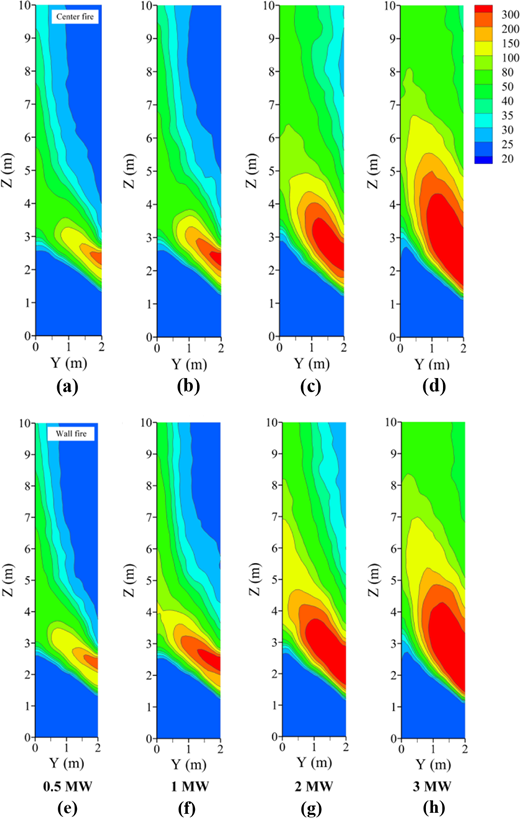
In a single-opening enclosure fire, the buoyancy-driven thermal smoke only flows into the shaft through the window, and consequently, a spill plume is formed. Figure 4 shows the temperature contours of the fire spill plume at x = 2.25 m in the shaft. For clarity, the complete computational domain is not shown, and only the local range from 0 to 10 m is showed for comparison. Figures 4(a-d) and 4(e-h) show the center fire and the wall fire, respectively. In the current study, although the fire outputs were set to the same HRR per unit area, four fires with HRR from 0.5 MW to 3 MW were used to represent the developmental process of the fire. As Figure 4 shows, the spill plume region grows as the HRR increases. At the initial stage (i.e. 0.5 MW), the thermal plumes from the burning compartment impinge on the sidewall facing the window and then spread along the sidewall to flow out of the opening at the ceiling. Next, the plumes gradually fill the entire upper space as the fire grows until forming flashover, as represented by the HRR of 3 MW. This means that more air needs to be entrained into the compartment from the bottom of the shaft. It should also be noted that the shaft is semi-open because the side at x = 4.5 m is not sealed, and thus, the lower part of the spill plume does not experience a significant temperature rise.
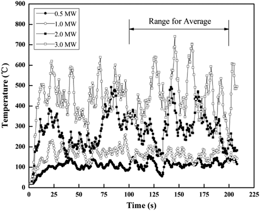
Based on the temperature contours, the influence of the HRR and fire location on the temperature distribution in the shaft cannot be effectively observed. Hence, the temperatures obtained with the thermocouples during the simulations are used for further analysis. Figure 5 shows the temperature history for TC 1, which is located at a height of 2.8 m. It can be observed that a greater HRR produces stronger temperature fluctuations, mainly because the air convection is enhanced as the fire grows. Also, Figure 6 shows that the temperature fluctuation decreases as the height increases. However, as shown in Figure 5, the values in the range of 100-200 s can be averaged to represent the temperature value for each specific height, which is conducive for making comparisons.
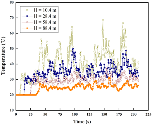
Temperature histories at different vertical heights for the center fire with HRR = 2 MW
Temperature histories at different vertical heights for the center fire with HRR = 2 MW
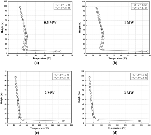
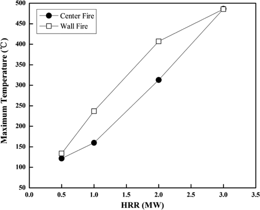
Figures 7 and 8 show the vertical temperature distribution in the shaft, and illustrate the influence of the HRR and fire location, respectively, on temperature distribution. As Figure 7 shows, the temperature trend initially increases and then decreases. Meanwhile, it can also be observed that the maximum temperatures for all of HRR values occur at a height of 2.8 m, and the maximum value increases significantly as HRR increases. The temperature then decreases rapidly after reaching the maximum. In addition, as Figure 8 shows, the temperature difference stemming from the fire location gradually decreases as the height increases. This may be a result of conduction loss to the wall and convective loss through interactions with cold air as the smoke moves along the shaft.
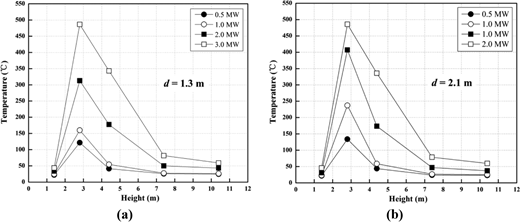
The maximum temperature values in Figure 7 are re-plotted in Figure 9 to analyze the effect of the fire location. It can be seen that the maximum temperature in the shaft increases with increasing HRR. In addition, the maximum temperature of the wall fire is greater than that of the center fire, which indicates that the constraint effect of the sidewall enhances the burn intensity. A possible reason for this is that more air is entrained from the shaft into the compartment through the window when the fire attaches to the sidewall. There is also a larger available space to mix well with air in the wall fire than the center fire, which causes more complete burning, and results in a greater temperature rise in the spill plume in the shaft.
To understand the flow state of the thermal smoke, velocity vector fields at x = 2.25 m in the compartment and shaft are shown in Figure 10. The flow field in the vicinity of the spill plume differs for the different fire stages, that is, with varying HRR. As Figures 10(a, b) show, an obvious feature is the occurrence of vortices in the shaft at a location near a height of 2 m, although these vortices fade away in Figures 10(c, d). Likewise, a similar phenomenon can be observed for the wall fire. In addition, the velocity fields in the compartment are more complex for the wall fire than the center fire, as can be seen by comparing Figure 10(g) to Figure 10(c). This may indicate that well-mixed burning can occur more easily when the fire is close to the sidewall than in a center fire. Another obvious feature observed in Figures 10(e, f) is that the thermal smoke mostly propagates along the left side of the shaft. Figure 10(h) shows that as the fire grows, the streamlines become uniform. This is because a larger fire produces higher temperatures, which results in a stronger buoyancy to drive smoke movement evenly in the shaft.
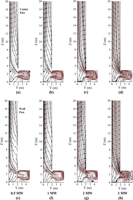
Figure 11 shows the velocity vector fields at y = 1 m. Because the right side is open, the airflow can be entrained from the surrounding area into the shaft. As Figure 11 shows, the streamlines incline to the left side, although this decreases as HRR increases. As a result, the high-temperature spill plumes from the compartment can gather one side of the semi-open shaft.
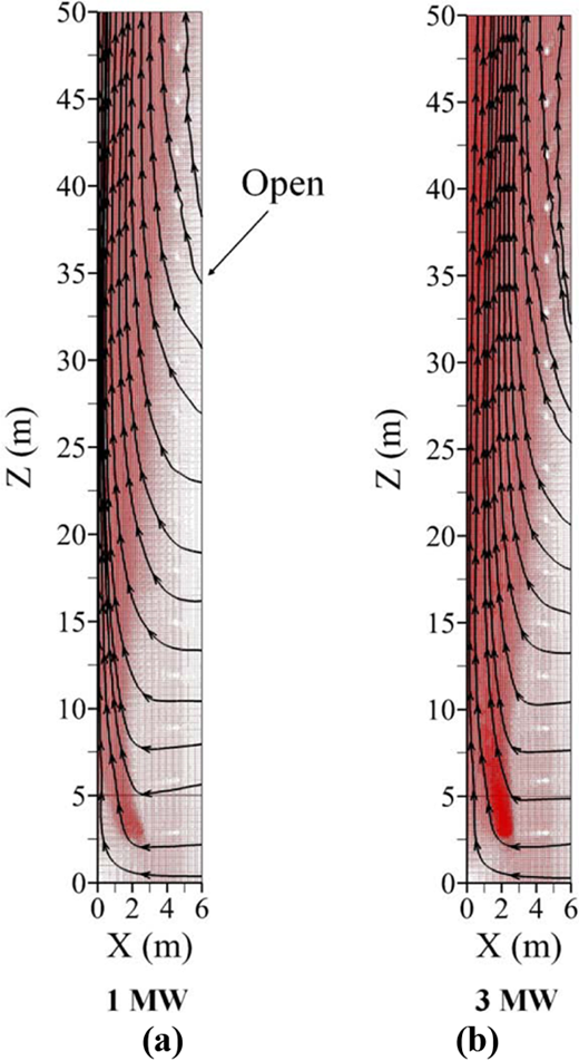
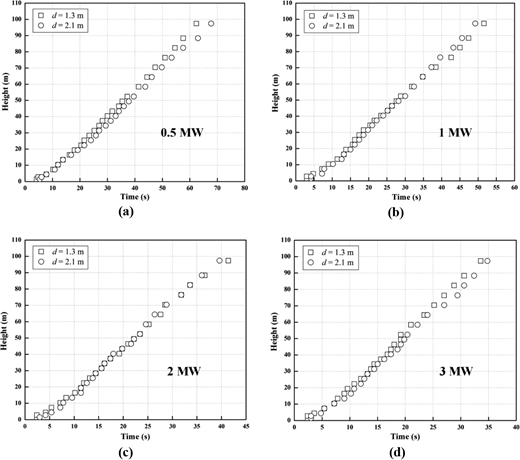
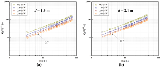
Figure 12 shows the rise-time relationship for the smoke plume front under different fire scenarios. As Figure 12(a) shows, the speed of smoke plume front at d = 2.1 m is slightly less than that at d = 1.3 m, as it takes the latter more time to reach the same height. A possible reason for this is that the flow path for the wall fire is longer compared than that for the center fire. On the whole, the influence of fire location on the rise-time of the smoke plume is weak, as shown in Figure 12(b, c). However, the difference in rise-time becomes significant as HRR increases. For the same fire location (e.g. d = 1.3 m), the rise-time decreases as HRR increases.
Based on analysis of Figure 12, it is clear that the rise-time of the smoke plume front, t, is dependent on the vertical height of the front, H, the horizontal distance between the fire center and the window, d, and the HRR of the fire source, Q. The dimensionless rise-time of smoke plume front, , is plotted against the normalized vertical height, H/d, in Figure 13 on logarithmic axes. The results show that is a power function of H/d with an exponent of 0.7. The fitted equation can be given as follows:
where g is the gravitational acceleration, and α is a constant coefficient.
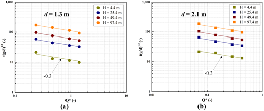
Likewise, Figure 14 shows the power function relationship between and the dimensionless HRR, Q*. The exponent is −0.3, and the fitted equation can be expressed as follows:
where β is a constant coefficient, and ρa, cp and Ta are the ambient air density, specific heat capacity and ambient air temperature, respectively. It should be noted that d is selected as the characteristic length in Equation (3) to consider the effect of different fire locations.
Combining Equations (1) and (2), the correlation between t, d, Q and H can be obtained for different fire cases as follows:
where λ is an integrated constant coefficient that can be obtained from the simulation data. The dimensionless rise-time of the smoke plume front in the shaft is plotted against (H/d)0.7Q*–0.3 in Figure 15.
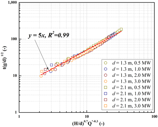
As Figure 15 shows, increases linearly with (H/d)0.7Q*–0.3. The resulting fitted equation can be given as:
Equation (5) can be used to predict the rise-time of the smoke plume front in a semi-open vertical shaft. Finally, a comparison of the simulation data with the rise-time calculated using Equation (5) was carried out, and the linear regression analysis is shown in Figure 16. The result show that Equation (5) provides fairly good predictions for the rise-time of the smoke plume front, and the maximum error is less than 20 per cent.
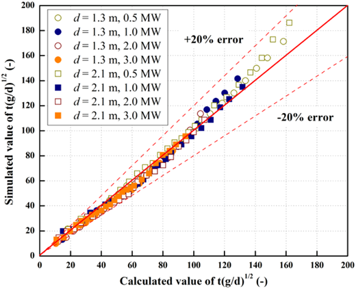
Comparison of the simulation results with values calculated using Equation (5)
Comparison of the simulation results with values calculated using Equation (5)
4. Conclusions
In this study, a set of full-scale simulations were conducted using the LES method to investigate the transport phenomena of fire-induced smoke flow in a semi-open vertical shaft. The effects of different fire locations and heat release rates on the temperature distribution and flow field were analyzed, respectively.
When the fire attaches to the sidewall, the burning intensity of the fire is enhanced, resulting in a larger continuous flame region in the compartment and higher temperatures of the spill plume in the shaft compared to a center fire. In the initial stage of the fire with a small HRR, the buoyancy-driven spill plumes incline to the side of the shaft opposite the window. Meanwhile, the thermal plumes are also moved away from the center of the shaft by the entrained airflow because one side of the shaft is open. However, the inclination diminishes as HRR increases because a greater HRR produces higher temperatures, resulting in a stronger buoyancy to drive smoke movement evenly in the shaft. On the whole, the combined effect of these factors could lead to the fire spill plume gathering on one side of the semi-open shaft. In addition, a dimensionless equation was proposed to predict the rise-time of the smoke plume front in the shaft.
