A GIS‐based climate change adaptation strategy tool

A large body of work exists on the potential impacts of climate change on the natural or man‐made environment. In general, the impact of climate change on biological systems represents a challenge requiring complex system modelling. Understanding the regional impacts of climate change on biophysical systems requires an analysis of global climate model (GCM) outputs, the cornerstone of the climate change research.

Currently GCM projections provide only coarse resolution information that is not suitable for local applications. Some form of regionalisation technique is required to translate the coarse climate change projections to a scale relevant for impact studies. However, providing regional climate variables is not the only challenge in tackling the impact of climate change on biophysical systems. Relevant climate indices that incorporate phenological knowledge are also required to transform climate change information into physiological information.

A holistic approach is required to incorporate the regional scale analysis of relevant climate indices. In general, in climate or systems modelling, the value of geographic analysis and spatial visualization is well recognised as it enables users to improve on the interpretation of modelling outcomes across an area or region. This spatial analysis enhances the limited applicability of single site simulation. For these reasons, the use of geographic information system (GIS) software is widespread. However, use of such software is challenging and many potential users are not equipped to take full advantage of the comprehensive spatial and visualization analysis features provided.

One way to improve the applicability and usefulness of GIS applications is to develop a simplified task‐specific system accessible by non‐GIS users, either incorporating GIS ActiveX controls (Smakhtin and Eriyagama, 2008) or embedded GIS software (Rao et al., 2000; Panagos et al., 2008; Liu, 2009). The usefulness of these GIS‐enhanced systems was demonstrated in the case of the sediment assessment tool for effective erosion control (SATEEC) developed to estimate soil loss and sediment yield (Lim et al., 2005). This tool can be used to identify areas vulnerable to soil loss and to develop efficient soil erosion management plans.

Such a GIS framework has the potential to provide an enhanced ability to assess the possible responses from a range of adaptation strategies to climate change. This enhancement can be archived by integrating the outputs from GCMs, downscaled to the local scale relevant for impact studies with various phenological modelling efforts that translate climate variables into indices relevant to agricultural industries. This GIS‐enhanced framework could enable scientists, policy‐makers and educators to evaluate climate change adaptation strategies and assist with communication of the impacts (Leal Filho, 2009; Mirfenderesk and Corkill, 2009).

The purpose of this work is to integrate knowledge relevant to climate impact management including the global climate response to a range of emission scenarios and how they translate to local scale climate variables and crop relevant indices based on appropriate statistical downscaling techniques. These analyses are incorporated into a stand‐alone GIS‐based risk assessment tool that is designed to enable an effective assessment of various adaptation responses for major agriculture sectors.

In this communication, after an overview of climate change adaptation strategy tool (CCAST), the GIS functionality which has been developed is succinctly described. A case study illustrates the use of the tool by describing the impact of climate change on wheat flowering and the response of plausible adaptation strategies. Finally, the portability and applicability of the tool to other industries and locations is discussed.

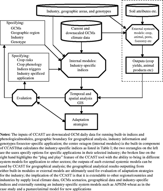
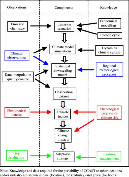
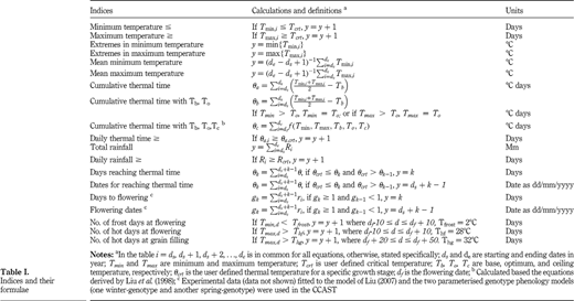
A schematic representation of CCAST (Figure 1) summarises the approach chosen and the required inputs. The components in Figure 1 that are bounded by the broken line demonstrate the “plug and play” feature of CCAST with the ability to bring in different system models for application to other sectors. The inputs for CCAST are current and future GCM‐projected daily climate data. Daily climate data for the current climate are downloaded from the SILO database (www.bom.gov.au/SILO) based on 1,062 observed sites across New South Wales (NSW). The key variables are daily minimum and maximum temperatures and rainfall amount. Future radiation data are generated by using the available climatic data (Liu and Scott, 2001). The radiation data is needed for running crop systems models such as agricultural production systems simulator (APSIM) for the case studies. GCMs are downscaled to each site for both the current climate and future projections. Additional input data is the map boundary data (longitudes and latitudes provided as text files) to enable the GIS display. Phenologically based climate indices for a specific industry is built in the tool. Currently, 20 indices (Table I) are available in the existing version of CCAST, which are tailored for the wheat industry. Their applications to different crops require setting their respective risk or phenological criteria or triggers as described in more detail in the following case study. The outputs of CCAST are the visualization of impacts of climate changes on a particular index over a user‐selected region. The geographical analytical results are ultimately used for evaluating adaptation strategies developed for the industry.

The application of CCAST for a different region requires the acquisition of appropriate boundary data as well as downscaled climate variables relevant for that region. As shown in the broken line frame of Figure 1, CCAST uses the outputs from any system simulation model of a specific industry. This function combined with these built‐in indices makes CCAST, a powerful tool for geographic analysis and spatial visualization of the impacts of climate change, applicable for on any ecological system. Finally, the existing version of CCAST uses current state‐of‐the‐art statistically downscaled GCM outputs, but the tool can use outputs of any other downscaled GCM data, if they become available. All these features ensure CCAST to be a highly flexible tool that can be used in all geographical areas of the world for any natural or man‐made environment.

Statistically downscaled climate data are obtained from the Australian Bureau of Meteorology (BoM)'s statistical downscaling model based on an analogue approach (Timbal and McAvaney, 2001) and available Australia‐wide including NSW (Timbal et al., 2009). Daily GCM data are extracted from the coupled model intercomparison project phase 3 (CMIP3) assembled as part of the intergovernmental panel on climate change (IPCC) fourth assessment report of climate change science released in 2007 (Solomon et al., 2007). Because daily data are required to perform the statistical downscaling, only 12 out of 23 GCMs were used. Daily climate data are available for three time‐slices: 40 years from 1961 to 2000 for the twentieth century simulations and two 20‐year periods from 2046 to 2065 in the middle of the twenty‐first century and from 2081 to 2100 at the end of the twenty‐first century. For future projections, two emission scenarios are considered (out of the six recommended by the IPCC (2000)): A2, a high emission scenario, and B1, a low emission scenario.

Basic climate indices such as temperature and rainfall or more complex indices as in Table I can be plotted for any single site across NSW using CCAST. In all cases, time series can be plotted from 1900 to 2000 using observations and compared with similar series from downscaled climate models (any of the 12 GCM‐used) over the period 1961‐2000 and for any period in the year or season. Prior to examining how these indices may change in the future, the user can evaluate the effectiveness of the statistical downscaling to remove known biases from the GCMs. These GCMs do not provide point specific information but rather large grid box averages. Therefore, residual biases for the chosen climate index at any particular location can be evaluated for any GCM and taken into account when the response to climate change for the same quantity is later analysed.

Once an index is selected, spatial analysis can be performed to obtain a pattern of changes across target regions. The impact of the GCM downscaled projections on that particular index (any combination of GCM, emission scenarios or period of the year) can be displayed. The GIS capacity of the tool is high. The graphics can be processed and displayed within seconds to a few minutes for a resolution of up to 500 m. For each case, the indices are calculated as cumulative distribution functions representing either the current observed period 1961‐2000 (I_mc), model based hind‐casting of the same 1961‐2000 period (I_hc), or future projections by 2050 (I₂₀₅₀) or 2100 (I₂₁₀₀), as well as changes for 2050 (ΔI₂₀₅₀) or 2100 (ΔI₂₁₀₀). In addition, downscaled model errors between I_mc and I_hc are also available. Apart from the observations based I_mc, all the other distribution functions are calculated for every individual GCM. As another useful feature of the tool, a specific percentile α (0≤α<0.5) can be set in the cumulative distribution function and attribute values in the corresponding four percentiles, α, (α+0.5)/2, 0.5, (1.5−α)/2, and 1−α can be extracted for plotting. A very large number of maps (up to 11,040 maps for one period of the year) are thus generated. This number increases further if more than one period, i.e. seasonal rainfall, or different crop varieties are analysed. It represents a vast array of information to detail the impact of climate change on the wheat cropping industry across NSW. In addition, wheat yields are simulated by APSIM‐wheat (Keating et al., 2003) and output from the external system model are read into CCAST for spatial analysis.

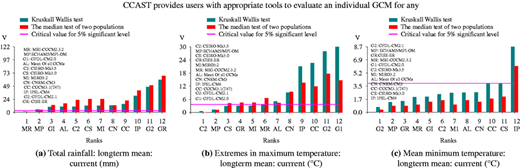
CCAST provides users with appropriate tools to evaluate an individual GCM for any specific climate index by comparing the distributions between the indices associated with the hind‐casting and the historical record. This allows for the selection of more suitable GCMs based on an end‐user perspective and the appropriateness of downscaled GCM to produce realistic industry relevant climate indices. In CCAST, when an index is selected, the performance of all GCMs for the selected index can be evaluated. The index calculated based on the GCM simulation of the 1961‐2000 time‐slice (hind‐cast) and that based on the historical record for the same period were considered as two populations and their differences tested with the Kruskal‐Wallis test and the Median test of two population (Kanji, 1993). GCMs were ranked based on the combined rank of the two χ²‐values (Figure 2). These rankings provide indicative information to users on the relative performance of each of the GCMs. GCM performance differs according to the variable of interest (e.g. typically rainfall‐based indices were less reproducible than temperature‐based indices). The results highlight the complexity of climate model evaluation. This is a non‐trivial task requiring spatial analysis of available models and several statistics. The innovative design of CCAST makes the evaluation of available GCMs able to be tailored to the end‐user applications. This opens up a new field of possible climate model evaluation alongside the more classical evaluation framework based on observed meteorological variables as used extensively in the state‐of‐the‐art climate science evaluation literature (Solomon et al., 2007).

Development of stand‐alone GIS functionality involves four major steps: implementation of map projection, determining boundary allocation, data interpolation, and a graphical display of the spatial data. They are briefly discussed below.

Mapping projection. The van der Grinten projection and Lambert projections are implemented in CCAST. The former was adopted by US National Geographic Society as their reference map of the world from 1922 to 1988 (Snyder, 1993) and the later was used by the NSW Department of Lands (Geocentric Datum of Australia 1994 (GDA94)). As the van der Grinten projection is neither equal‐area nor conformal, we implement the Lambert conformal conic projection as well as the Lambert azimuthal equal‐area projection as an alternative. The two standard parallels for the GDA94 Lambert projection are −30°45′00″ and −35°45′00″. The alternative mapping projections are included as the tool has potential for use beyond NSW, Australia.

Boundary. It is assumed that a boundary dataset is a set of limited points enclosing a geographical area of interest. The boundary is approximated as a set of joined linear lines between each two neighbouring points.

Interpolation. Inverse distance weighted (IDW) and Kriging interpolations are implemented in CCAST.

IDW is a simple and easy interpolation method for predicting unmeasured values. This method uses the weights directly calculated from the inverse of powered distances: Equation 1 Where k=1, 2, 3 … , d_i,p is the distance between the observed point i and the predicted point p; Z is the value of the indices. Notice that if k=0, equation (1) becomes an interpolation which is calculated by the simple mean of nearby points. The main disadvantage of this method is the arbitrary definition of the interpolation which is directly related to distances (Mueller et al., 2005).

Kriging interpolation. In this scheme, interpolation is based on semi‐variances which are calculated as: Equation 2 where n is the number of pairs of sample points separated by distance d (called lag distance), z(x) and z(x+d) are the data values at the two‐paired locations. The relationships between the semi‐variance and the lag distances are often nonlinear. In CCAST, 13 equations are included for nonlinear regression of the semi‐variance relationships. These equations include spherical, exponential, Gaussian models and their derivatives which have no intercepts.

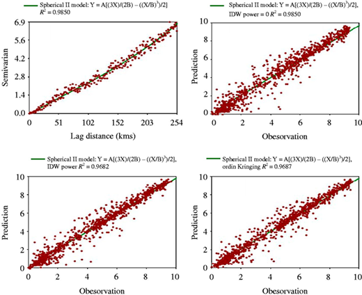
For each selection of indices, the relationship between semi‐variance and lag distance can be evaluated and the best fitted relationship is used for interpolation. To assist the selection of the best interception scheme, Kriging with the best fitted equation and IDW interpolation methods were validated by leave‐one‐out cross validation (Wilk, 1995). The power of k=0, 1, 2, … 8 of IDW, ordinary Kriging and universal Kriging interpolations are compared by a number of statistical variables such as correlation coefficient (R²) and root mean squared errors.

To illustrate the validation of the interpolation methods, changes in the long‐term annual averaged number of hot days are briefly discussed. The relationship between semi‐variance and lag distance is well described by a modified spherical equation (no intercept) with a R² of 0.986 (Figure 3). Cross validation showed that the ordinary Kriging interpolation gave the best result of R²=0.969, compared to IDW (p=3) with an R²=0.968 which is the best interpolation over all nine IDW interpolations. It also showed that IDW (p=0) gives an R²=0.959, suggesting that even a simple mean of observations from nearby sites can give a good interpolation. Similar results can be obtained for other climate indices.

Graphical display. Neither external plotting controls nor software is used in CCAST. Displaying the spatial data is achieved by using the “print” or “line” property of picture controls in VB 6.0. All GIS data including, mapping projection, boundary positioning and interpolation are calculated within CCAST.

As a case study, wheat flowering is modelled by a phenological model as described by Liu (2007) with two parameterised genotypes, which require the computation of several indices (Table I). The inclusion of this phenological modelling within CCAST via the computation of relevant climate indices highlights how climate change projections will spatially alter flowering dates and the sensitivity of these spatial variations to emission scenarios and climate models. The two contrast genotypes are spring and winter genotypes. These were used to demonstrate the tool's potential, but the tool has been designed in such a way that it allows for a similar analysis for a range of other winter and/or summer crops.

The potential impacts of climate change on wheat crop production across NSW is analysed using CCAST. In order to provide guidance for an adaptation strategy for future wheat cropping systems, simple phenological models for two contrasting wheat genotypes are included. The phenology models and parameterisation procedures are explained in detail by Liu (2007). Briefly, the rate of progress towards flowering, r_i, is given by: Equation 3 where r_i ≥ 0, T_i is the mean temperature of the day and P_i is the photoperiod of the day, b₀, b₁, and b₂ are coefficients given in Table II. The vernalization function, f(v_i), is calculated by the equations (1)‐(4) of Liu (2007), where the values for v_f (Table II) and three cardinal temperatures, T_l,v, T_o,v, and T_h,v are required. The values of −1.3, 4.9 and 15.7°C, respectively, for the three cardinal temperatures are used. The indices used for the case study of the impacts of climate change on wheat flowering are:

d_h number of days when T_max>28.0°C or heat stress days for winter cropping;

d_f, number of days when T_min<2.0°C or equivalent to frost days in field; and

f, flowering date, when at 50 per cent wheat heads are flowering.

d_h and d_f are analysed for the period from 1 May to 30 November and flowering period was defined from f−10 to f+10 days. The flowering data is the day when the summation of daily developing rates (r_i) is greater or equals to 1.0 from the date of crop sown.

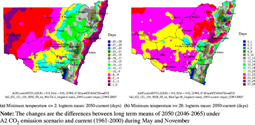
Frost occurrences by 2050 are projected to decrease by up to 29 days (Figure 4(a)), with a decline in excess of 12 days for almost 80 per cent of the state. These numbers are based on a single GCM using the A2 emission scenario. The chosen GCM is evaluated as the best performer across the three climate indices (d_h, d_f and f) chosen in this case study. It is important to note than in order to obtain a physically consistent future climate, it is not advisable to pick different GCM for different indices. Therefore, in order to sample model uncertainties and to obtain more robust projections, several GCMs should be used, which consistently performed well in the reproduction of the chosen indices for the hindcast 1961‐2000 periods.

During winter crop growing periods, hot days are projected to increase by 2050 by up to 28 days, but 90 per cent of NSW state are projected to have 12‐28 days more hot days by 2050 (Figure 4(b)). The projected increases in hot days show two distinct regimes: a coastal strip east of the great dividing range and the remaining area in‐land. Increases in hot days are expected to be <16 days along the coastal strip but are projected to be 16‐29 days in‐land.

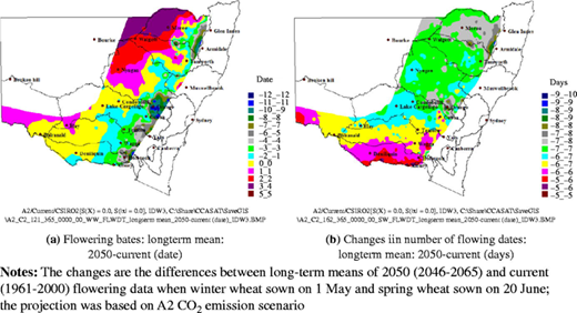
Currently, wheat flowering time in the NSW wheat belt ranges from mid September in the north‐west to mid October in south‐east of the NSW wheat belt. The flowering time of the two contrasting genotype wheats is simulated to be well within the current flowering time (data not shown). By 2050 under an A2 CO₂ emission scenario projected by CSIRO‐Mk 3.5, the flowering time of the winter genotype varied from five days later in the north west to 11 days earlier in the central tablelands (Figure 5(a)), while the flowering time of the spring genotype is within 4‐7 days earlier than current timing across NSW (Figure 5(b)). The winter genotype in the current cool environment will flower earlier as there will still be sufficient cool conditions for completion of vernalisation in the projected future climate, and the projected warmer conditions will promote crop flowering. However, in the currently warm areas, further warming will result in insufficient periods of cool temperatures for vernalisation and hence flowering time of the winter genotype wheat will be delayed. As spring wheat genotypes do not require vernalisation, the warming conditions will make the crop flowering consistently earlier across the whole wheat belt of the state.

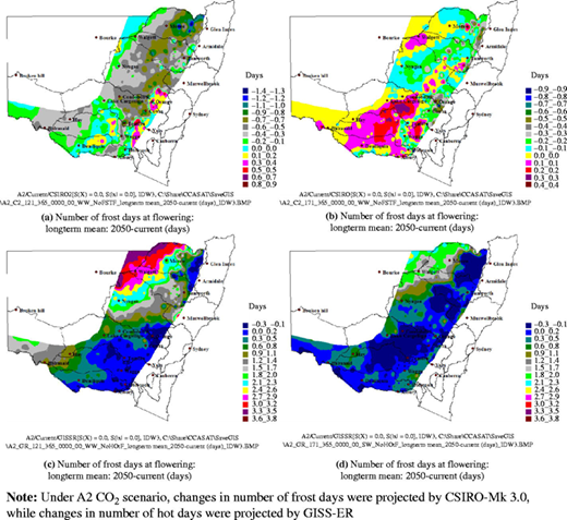
Figure 6 shows that in a future climate under an emission scenario A2, the number of frost days during flowering period of both winter and spring wheat are projected to be slightly changed, ranging between −1.0 and+0.5 day for winter wheat and −0.6 and+0.3 day for spring wheat, on average. CSIRO‐Mk 3.0 projection is used as it is the best performing scenario for changes in number of frost days. However, under the same emission scenario, hot days during flowering time could be up to five days more for winter wheat and two days more for spring wheat, according to Goddard institute for space studies (GISS)‐ER. About 30 per cent of the NSW wheat belt is projected to experience ≥2 days more hot days on average, during the flowering period of winter genotype wheat. However, only 2 per cent of NSW wheat belt is projected to experience ≥2 more hot days, on average, during the flowering period of spring genotype wheat. Therefore, the impact of climate change on the spring genotype is low.

CCAST is a stand‐alone GIS framework designed in a user‐friendly manner for non‐GIS skilled users. This is achieved by coding the tool exclusively in VB6 without inclusion of any ActiveX GIS controls nor embedded external GIS software. The tool can be used for analysing climate impacts, identifying the risks and opportunities that will need a response, defining the agricultural and geographical areas most sensitive to climate change and identifying appropriate adaptation responses. Statistical tests of GCMs performances are provided to help users to select the most suitable GCMs for their specific indices. The tests are based on spatial analysis. Such tests are not available in most commercial GIS software due to computing limitation but with the GIS‐enabled CCAST, it will only take seconds to complete the spatial analysis of all available GCMs and present the results both in graphics and in a tabular format.

The tool does not rely on any database boundary, and can easily be ported to other locations in Australia or other countries. CCAST represents a novel approach and a state‐of‐the‐art development as it integrates a broad knowledge base relevant to climate change impact and adaptation (Figure 7). Relevant knowledge included estimating the possible future emissions scenarios based on economical and social development, the core physical science of the global climate response to external forcings, the applied phenological knowledge necessary to describe the interaction between the climate and the targeted agricultural industry. The tool also includes an advanced regionalisation technique to allow for a downscaling of the climate model large‐scale outputs to the local scale relevant to evaluating climate impact for a particular industry.

However, CCAST is not a simulation model as shown in Figure 1, but it is designed to use the outputs of any system simulation model for analysing impacts of climate change and evaluating adaptation strategies for an industry of interest. Although it includes some basic climate indices and modules for crop development, it is not necessary or possible to enclose all system models within a tool. The feature that can utilise the outputs of any simulation model enables CCAST a powerful tool as it can be easily extended to any new industries, where their system models can readily run over a spatial context.

This paper demonstrates the usefulness of the GIS features embedded in CCAST using industry‐specific indices to visualise the impacts and develop adaptation strategies to climate change. A case study using the tool showed that the number of frost days in a future climate is not projected to change dramatically, however, projected increases in hot days during wheat flowering time will be a serious problem. Selecting suitable wheat genotypes is the key adaptation strategy for managing the impacts of climate change on wheat cropping. Spring wheat genotypes appears to be more suitable in projected future climate over most areas, while winter genotypes are projected to remain appropriate in limited areas where sufficient periods of cool temperature exist for completion of vernalisation. Breeding strategies should, therefore, focus on releasing varieties that do not require vernalisation, but can be sown early in the season.

The development of CCAST was funded by a NSW Government Climate Action Grant administrated by NSW Department of Environment and Climate Change. The authors wish to acknowledge useful comments received from technical reference panel members, specifically, Dr Peter Hayman (South Australian Research and Development Institute, Australia) and Dr David Jones (Centre for Australian Weather and Climate Research, Bureau of Meteorology, Melbourne, Victoria, Australia), during the life of the project.

De Li Liu is a Senior Research Scientist in the NSW department of Industry & Investment based at Wagga Wagga, New South Wales. De Li holds a BSc in Agriculture and a PhD in Rural Science. He has developed a number of decision support systems and models used by researchers, advisors and farmers. De Li's area of interest includes the climate change impact analysis and adaptation research in agricultural systems. De Li Liu is the corresponding author and can be contacted at: de.li.liu@industry.nsw.gov.au

Bertrand Timbal is a Scientist with the Australian Bureau of Meteorology (BoM) based in the Centre for Australian Weather and Climate Research (CWACR) – a joint partnership between the CSIRO and BoM. He has more than 15 years experience dealing with climate change simulations and developing methodologies to provide local scale information relevant to impact studies, including the statistical downscaling model used in this application.

Jianhua Mo is a Senior Research Entomologist in the Department of Industry & Investment based at Yanco, NSW. Jianhua Mo holds a BSc and MSc in Agriculture and a PhD in Forest Entomology. He has studied the population ecology and management of a number of agricultural and forest insect pests, including modelling the impact of climate on insects and crops.

Helen Fairweather is currently the Manager of Coastal Impacts within the Queensland Climate Change Centre of Excellence (QCCCE). QCCCE is within the Office of Climate Change, which is a unit within the Queensland Department of Environment and Resource Management. QCCCE has a role to deliver the climate change science to underpin the policy being developed by the Office of Climate Change. Helen's area of interest is in the impact of climate change on the flood risk in Queensland and the interaction with sea level rise and storm tide inundation. Prior to her current position, she was a Research Leader of the Climate Science Unit of NSW Department of Primary Industries – present Primary Industry Branch of Industry & Investment NSW.