Integration of climate change and land‐use scenarios in nutrient leaching assessment

Since the early 1900s, the Baltic Sea has become increasingly eutrophied as a result of increasing inputs of nitrogen and phosphorus from anthropogenic activities in the catchment area and at the sea. Despite the practical efforts to reduce the emission of nutrients, the implementation of river basin management measures as envisaged in the EU water framework directive (WFD) is still deficient (EEA, 2010).

Modelling future land‐use and environmental problems are not new research fields. The first urban land‐use models were developed to simulate the historical development of cities. In recent decades, focus has been put on modelling either the urban land‐use development (Clarke et al., 1997; Barredo et al., 2003; Solecky and Oliveri, 2004) or the agricultural land development (Verburg et al., 2002). Attempts to model both urban and agricultural development simultaneously are still rare, but they do exist (Rounsevell et al., 2006; Verburg et al., 2006).

Several models have been developed for modelling environmental phenomena related to hydrology and to the nutrient cycle. Examples of these are the GWLF and INCA models (George, 2010; Puustinen et al., 2010). With the aid of different models, the influence of climate change on the nutrient loading has been studied (George, 2010; Rankinen et al., 2009). Climate change is likely to increase nutrient loading (Silander et al., 2006), having a harmful impact on water quality. More research on the combined effects of land‐use and climate change on environmental issues, such as the leaching of nutrients, is however needed to support river basin planners in their future‐oriented tasks.

The objective of the current paper is to describe an integrated modelling approach for studying the combined effects of changes in land‐use and climate using regional IPCC based land‐use and climate scenarios. The aim is to analyse the leaching of phosphorus at regional and local scale with an easily understandable and environmental planner friendly modelling framework. In addition the paper reflects on the added value of a geospatial data based modelling approach from a river basin management perspective.

This paper is divided into six parts. After this introduction, the study area is introduced, followed by a description of the methodological framework. It includes a description of the emission scenario framework, the land‐use model, the nutrient leaching model and the main data applied. Section 4 presents the results of the variable and scenario construction and of the nutrient leaching modelling. The results are discussed in Section 5 and the paper ends with some conclusions.

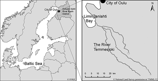
The WATERPRAXIS project during 2009‐2012 focused on developing water management practices for selected pilot sites around the Baltic Sea Region (www.waterpraxis.net). One of the pilot sites was the River Temmesjoki river basin, which is part of the Oulujoki‐Iijoki river basin district (RBD) in Finland (Figure 1).

Oulujoki‐Iijoki RBD is predominantly a rural area, covering 68,085 km². The municipalities in the Western part have been affected by the economic growth of the city of Oulu. Thus, the population growth rate was one of the highest in Finland for the last decade: for example the population in Liminka municipality increased by 49.5 per cent from 5,735 in year 2000 to 8,576 in year 2008.

The River Temmesjoki is situated in the commuting area of the city of Oulu in the municipalities of Liminka and Tyrnävä. The length of the river is 75 km and its drainage area is 1,181 km². In year 2010 there were 12,000 inhabitants in the drainage area. The majority of the inhabitants live in the municipality centres of Liminka and Tyrnävä, while the remaining population lives in scattered settlements mainly along the river network.

The River Temmesjoki river basin is, in a Finnish context, a very intensively cultivated drainage area. It is covered to 19 per cent by agricultural land, which is mainly situated in the lower parts of the basin. Forest and bog areas dominate in the upper parts of the river basin. The concentrations of nutrients and suspended solids are very high and the ecological status of the main river channel is poor according to the definition of ecological status as defined by the WFD (EC, 2000). The River Temmesjoki has two tributaries: River Tyrnävänjoki and River Ängeslevänjoki, which have a poor and a bad ecological status (www.ymparisto.fi/download.asp?contentid=111567&lan=fi). The River Temmesjoki discharges to the Liminganlahti bay, which is an internationally significant bird and nature conservation area. Environmental planners face a big challenge to meet the goals of the WFD for the River Temmesjoki. Due to its present poor ecological status and rapid land‐use change it is imperative to study and analyse the combined effects of land‐use and climate change in this area.

Scenarios are suited for studying optional developments and uncertainties (Koomen et al., 2008). The Intergovernmental Panel on Climate Change (IPCC) has developed a framework of emission scenarios referred to as the special report on emissions scenarios (SRES) that correspond to the storylines and driving forces used by IPCC (Nakicenovic et al., 2000). The SRES framework proposes four major equally possible scenario families; in the A scenarios, the world will face an economic‐driven future, where focus is on material wealth and where the challenges of today will be solved by technological innovations rather than by changes in lifestyle, while in the B scenarios, the future is driven by the concern of environmental, social and economic sustainability. In the SRES scenarios of type 1, i.e. A1 and B1, the solutions are of a global nature, while in the SRES scenarios of type 2, i.e. A2 and B2, the emphasis is on regional solutions. The SRES scenario framework is coarse in scale, generic and qualitative and does not include guidelines on how to apply it on regional scale (Rounsevell et al., 2005).

Land‐use is strongly interrelated with the development of the society, i.e. the spatial land‐use structure of an economy‐driven world will on regional level look very different from a land‐use structure in a world driven by socio‐economic equality and environmental concern (Rounsevell et al., 2006). In land‐use scenarios corresponding to the A families, built‐up areas are expected to expand along road corridors and around peri‐urban centres, continuing the car‐dependent development of today. Spatial planning is also expected to be weak (Solecky and Oliveri, 2004; Verburg et al., 2006; Hansen, 2010). In the B scenario families new built‐up areas are expected to emerge in a compact manner along edges of and within existing settlements, with only minimal spontaneous growth taking place (Solecky and Oliveri, 2004; Verburg et al., 2006; Hansen, 2010). To be able to analyse the environmental effects of different SRES scenarios on regional level, land‐use that correspond to different SRES scenarios need to be simulated. A land‐use model can help simulating future land‐use changes.

Rounsevell et al. (2006) and Verburg et al. (2006) used land‐use models to produce land‐use scenarios corresponding to the SRES framework on European scale, taking into account both the development of urban and agricultural areas. Due to the regional scope of the current study, it was decided to use the land‐use change impact analysis (LUCIA) model (Hansen, 2007). LUCIA is based on multi‐criteria evaluation and cellular automata, and the model has been used in other regional land‐use studies (Hansen, 2010, 2012).

Regular factors, such as proximity, accessibility and suitability are included (Hansen, 2007; Barredo et al., 2003), but no factor is compulsory. In LUCIA, the proximity factor is derived statistically for the active urban classes from the land‐use time series using a neighbourhood rule metric explained in Hansen (2012). Whereas, the primary active land‐use classes (urban) demonstrates a rather complicated neighbourhood interaction with ten distance zones and by involving many land‐use classes, the neighbourhood interaction for the secondary active classes is simpler. Generally it is convenient for the farmer that new fields are located adjacent to existing fields to facilitate optimum use of the whole area. Accordingly, the neighbourhood interaction for the active secondary land‐use classes only considers the eight adjacent neighbours when assessing the neighbourhood effect. Thus, a new farmland cell will be located where a majority of the adjacent cells also is used for farmland.

There is an option to include a yearly changing random factor, which introduces some random noise to the simulation. The random factor can be used to represent the fact that land‐use changes are based on decisions taken by individuals or groups of individuals and are affected by land ownership and price, i.e. factors on which there often is no spatial information available. There is also an option to include three user‐defined additional factors in the simulation. The flexibility the user‐defined factors offer is of great value, when the aim not only is to reproduce the historical land‐use development, but also to produce alternative non‐linear scenarios of the future.

LUCIA also integrates policies and legislation that have a spatial dimension. These variables are referred to as constraints. All factors and constraints are organised as a multi‐criteria evaluation. By combining the factors and constraints for each active land‐use type, the transition potential of each cell for changing from one type of land‐use to another can be estimated. The potential for each cell to change land‐use type at the next time step is given by the function below: Equation 1 where P is the transition potential, C – constraints (values between 0.0 and 1.0), F_i – factors (values between 0.0 and 1.0), w_i – individual weight factor between 0 and 1, and L – land‐use type. Initially w_i is set to 1.0 for all factors, but during calibration the value of w_i can be lowered to obtain a better agreement between the simulated land‐use and the real land‐use change for historical years (Hansen, 2007).

Land is generally devoted to the use that generates the highest potential profitability. Since urban land‐use takes priority over agricultural production (Verburg et al., 2006; Rounsevell et al., 2005), the urban expansion first reserves the number of cells that it needs from the passive or secondary active land‐use classes. Next the secondary active land‐use classes or in this case agriculture takes it share (Table I). The passive land‐use classes are mainly represented by different kinds of natural vegetation, such as forest and wetland. The static classes remain unchanged during the simulation.

Simulation of future land‐use involves a wide range of data that have to be obtained and pre‐processed. The most important data are temporal land‐use datasets. Temporal land‐use data are useful for model calibration purposes, for factor validation and for quantifying the land‐use demand based on historical land‐use changes (Sohl et al., 2010). The temporal land‐use data is also useful for examining recent spatial changes in the area to be modelled. Analysis of the observed changes in land‐use can assist in refining the downscaling methodologies used in scenario construction (Rounsevell et al., 2005) and in better understanding the characteristics and region‐specific development options at hand.

To explore recent land‐use changes, consistent land‐use time series were compiled. First raster datasets representing the built‐up areas for the years 2000, 2002, 2005, 2007 and 2008 were produced. The built‐up areas were classified into residential, service and industrial areas using 250‐m resolution data from “the monitoring system of spatial structure” (www.ymparisto.fi/ykr). The building type with the highest number of buildings was allocated to a particular raster cell. To capture the spatial expansion of built‐up urban cells and to ensure data consistency, the built‐up datasets were aggregated with the previous datasets, i.e. so that the built‐up dataset of 2002 included both the built‐up cells from year 2000 and 2002 and the built‐up dataset of year 2005 included the built‐up datasets of years 2000, 2002 and 2005 and so on. Isolated, alone standing built‐up cells were excluded from the aggregated datasets. The criterion for exclusion was that a built‐up cell had to have at least one built‐up neighbour in its Moore neighbourhood of eight cells to be included in the aggregated data series. Finally, the aggregated built‐up datasets were combined with Corine land cover (CLC) data for year 2000 of the same resolution to produce land‐use datasets of a consecutive series of years.

According to agricultural statistics, the agricultural areas, that obtain subsidies, have increased from 229,000 hectares in year 2000 to 253,000 hectares in year 2007 in the study area. This corresponds to a yearly increase in agricultural areas of 3,428 hectares. To capture the land‐use changes related to agricultural expansion, information from the CLC change (CLCC) dataset and the “Finnish land parcel identification system” (FLPIS) were used. The CLCC dataset contains over one‐hectare changes between the CLC2000 and CLC2006 in 25‐m resolution. FLPIS again contains the geometry of the field parcels and information on its major crop type. Information from the FLPIS representing year 2007 was used to classify each field parcel according to its main crop; cropland, grassland or root vegetables. Available parcel data did not cover all of the agricultural cells in CLC 2000 and in the CLCC, since also the unsubsidised agricultural areas are included in CLC. The 25‐m resolution FLPIS data was expanded by 50 m in order to allocate a value to the agricultural cells, which are missing a crop type. The remaining agricultural cells that could not be classified using this method were included in the grassland class. The FLPIS data was not available for year 2000. The major crop type was therefore assumed to have stayed the same and the field register dataset was used to allocate the main crop type also to the field pixels of the land‐use data of year 2000.

Based on the temporal land‐use data, the demand for the active land‐use classes were set in LUCIA. The demand for the active urban land‐use classes was based on the observed expansion of urban land‐use categories. These changes were translated into the average number of cells to change per active urban land‐use class per year and municipality. The numbers were extrapolated linearly into the future, estimating the demand per municipality and active land‐use category until the end of this century. This demand was altered for the active urban – residential, service and industry – classes using official population projection data. The statistics of Finland has made population projections on municipality basis until the year 2040. The demand for the urban classes was expected to correlate with positive population growth, so that the land‐use demand is higher in municipalities of positive population growth.

For the secondary active agricultural classes, the average yearly increase of agricultural cells is expressed in per mille. The agricultural land‐use demand is expressed as numbers of cells per municipality and active agricultural category. The total amount of cells to turn into new agricultural cells is related to the amount of agricultural cells at the baseline year in each municipality. When agricultural demand is included in the simulation, new agricultural areas will emerge. The agricultural demand functions as a feedback mechanism, so that new agricultural cells emerge elsewhere, to partly or completely compensate for the agricultural areas taken up by the built‐up area expansion.

Land‐use induced diffuse loading plays an important role in deteriorating water quality. RiverLifeGIS (RLGIS) is a nutrient leaching model with which one can perform hydrological and water quality related computations in a transparent and easily understandable way. In RLGIS, the nutrient loads can be estimated based on runoff and the relative abundance of a particular land‐use class (Karjalainen and Heikkinen, 2005). Unlike many other hydrological and nutrient related models, RLGIS is spatially fully distributed, which is relevant for this paper.

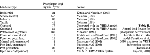
In RLGIS an estimate for the total land‐use originated diffuse loading is calculated based on land‐use data and on specific load figures for different land‐use types (Table II) using the following equation: D=ΣE_i*A_i, where D is the land‐use – originated diffuse loading (kg year⁻¹), E_i is the export coefficient for land‐use class i (kg km⁻² year⁻¹) and A_i is the area of land‐use i in the drainage area (km²). These estimates do not include any nutrient processes in the river (e.g. adsorption or mineralisation), only dilution. Therefore, the water quality modelling does not offer any new information about the nutrient dynamics in the situation of climate and land‐use change. However, this is not an objective of this study.

Flow directions are needed to calculate the flow and the phosphorus (P) concentrations. In RLGIS, the flow directions were computed using specific runoff (l s⁻¹ km⁻²) values. Flow directions were computed for each 250 m grid cell from a digital elevation model (DEM). Each grid cell may flow only to a neighbouring cell, so there are eight possible flow directions (N, NE, E, SE, S, SW, W, NW). Flow in different points of the flow network was calculated as follows: FlowA=A/B*FlowB, where FlowA is the flow in a point of interest, A is the upper catchment area of the point of interest, FlowB is the flow at a measurement point and B is the upper catchment area of point B.

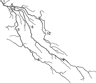
Since RLGIS is a spatially distributed model, where all calculations are performed in every grid cell, it is possible to derive P concentrations in every grid cell for example along a river network based on land‐use and flow (Figure 2). The average concentrations of P were modelled in milligram per liter using the average annual P loads and the average runoff values based on the input data described next.

P loads and concentrations for land‐use in 2007 and in 2040 were computed based on land‐use specific load figures (Table II) derived from literature and based on runoff values produced by the FINESSI project (Carter et al., 2004).

In Table II, conspicuous is the high specific load values of the service and potato land‐use types. The high values can be explained with the fact that service areas are the densest built‐up areas in Finland. Residential areas are not densely built in Finland on average and especially not in small municipalities like Liminka and Tyrnävä. The P load for potato (root vegetables) is comparatively much higher than for cropland and grassland, due to the heavy use of fertilisers.

Annual P loading is not expected to change significantly due to climate change (Kallio et al., 1997; Bouraoui et al., 2004; Tang et al., 2005). Due to this and to the objectives of this paper the same loading coefficients were used for calculating loading from the land‐use scenarios. The loading figures were slightly increased in calibration. Exact correspondence between computed and measured P concentration was not considered necessary, since scattered settlement and small point load sources were not included in the computation and since only changes in land‐use originated loading were studied.

Land‐use data of year 2007 and average annual runoff figures for the period 1961‐1990 were used to represent the nutrient loading of the baseline year 2007. The control runoff period was 1961‐1990, since it is the commonly used reference period in the scenarios of IPCC. Average annual and seasonal runoff data modelled by the FINESSI project to correspond to the SRES A2 and B2 scenarios of the time period 2040‐2069 were also used. To produce this 10 km resolution runoff data representing the baseline and the A2 and B2 scenarios, the hydrological modelling system of the Finnish environment institute had been used in conjunction with the global circulation models (GCM) HadCM3 (Had), ECHAM4/OPYC3 (EH4) and NCAR/PCM (NCAR) (Posch et al., 2008). These three GCM projections all fulfil the quality criteria of IPCC and they are all described in the Third Assessment Report (www.ipcc‐data.org/sres/gcm_data.html).

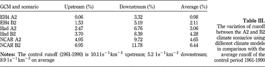
The average runoff values do not vary very much between the emission scenarios in the River Temmesjoki river basin. Runoff is only 1‐2 per cent higher in the B2 scenarios than in the A2 scenarios. Different GCMs introduce more variety. Average forecasted runoff from the River Temmesjoki river basin increases on average by 1‐2.1 per cent according to EH4, 3.1‐4.3 per cent according to Had and 4.7‐6.4 per cent according to NCAR. At some locations downstream, runoff increases by over 6 per cent (Table III).

The objective of the variable production was to produce a set of input data representing suitable factors and constraints to include in the land‐use model calibration and scenario simulation. Current research was carried out in cooperation with the regional body in charge of implementing the WFD in the study area. Environmental planners participated in the scenario making process by attending several working meetings, in which it in the end was decided, which land‐use scenarios should be produced and based on which factors and constraints. The quantitative model calibration and the choice of factors and so on were in this way supported by a qualitative approach.

The proximity factor was derived statistically for the active urban classes from the urban land‐use data series of the years 2000, 2002, 2005, 2007 and 2008 in LUCIA. The proximity factor for the agricultural classes was derived by comparing datasets from year 2000 and 2007.

The dataset representing the suitability factor was produced from existing land‐use data, by observing on which kinds of land‐use the land‐use changes has taken place for each active land‐use class. The relative presence of land‐use classes was taken into account. Generalised slope data was found useful to explain the placement of agricultural cells. The majority of the agricultural cell could be found in areas of <3 per cent slope. A dataset representing the slope factor was therefore produced.

The detailed road network correlated well will the placement of new built‐up and new agricultural cells and this is why it was chosen to produce the accessibility factor dataset. Of all cells in the study area, 26.6 per cent were within 250 m of a road. 81.58 per cent of the new residential cells had emerged within 250 m of a road. For new industry and service cells the percentage was even higher: 82.59 and 84.09 per cent. New agricultural areas do not seem to be as dependent on the road network, since 45.35 per cent of the new agricultural cells have emerged within 250 m to roads.

The distance to water bodies explained the spatial structure of new residential and agricultural cells well in the study area, and therefore an attractiveness factor was made based on the distance to water areas. For historical reasons, the settlement pattern in the Western parts of the study area follows the coastline and the rivers and streams. In the eastern parts the settlements are situated close to lakes. The trend to build close to water is continuing today; 74.83 per cent of all new residential houses were placed within a 500 m zone from water areas and the figures are almost the same for the service buildings (73.16 per cent), probably since service is often built in conjunction with residential housing. For the industry class the effect of the water is less or 64.44 per cent. The trend to build close to water areas is likely to continue also in the future, if regulation continues to allow it. New agricultural cells have emerged close to built‐up areas, which in turn can be found close to water. Of all new agricultural cells 60.26 per cent has emerged within 500 m from water bodies. Generally cropland is situated closer to built‐up areas than grassland.

The impact of different spatial constraints on the built‐up and agricultural development was also analysed. The placement of new built‐up cells was compared with the spatial extent of the Natura 2000 areas. Of all new built‐up cells only 8.32 per cent situated inside Natura 2000 areas during the study period. 99.19 per cent of the new agricultural cells are situated outside Natura 2000 areas.

Land‐use plans at regional and municipal level should steer building activities. Data representing the prevailing planning situation was compiled. The spatial analysis showed that 86.8 per cent of the new residential cells, 64.2 per cent of the new industrial cells and 71.4 per cent of the new service cells had emerged outside the planned areas.

To ensure the comparability of the results and to be able to specifically relate to changes in nutrient leaching due to differences in the land‐use structure, main focus was decided to be put on producing land‐use scenarios with identical urban demand for the A and B scenarios. To study the effect of changes in demand and to test the sensitivity of the results, scenarios where the urban demand was set to increase by 10 per cent in A2 and to decrease by 10 per cent in B2 were also produced.

The development options for agriculture are twofold in the study area according to the involved stakeholders. Agricultural areas can shrink, due to urban expansion and to changes in agricultural policy. Alternatively the agricultural areas will continue to expand because of regional protectionism, subsidies and due to improving climatic conditions. It is however expected the total area of agricultural land will stop increasing due to changes in the national part of the agricultural subsidiary programme, which presently sets restrictions on gaining subsidiaries for newly cleared agricultural land. Therefore, agricultural areas are not expected to increase in total, but it is at its maximum expected to stay the same in Oulujoki‐Iijoki river basin in relation to the baseline year in 2007; in the land‐use modelling approach used it means that the amount of agricultural areas taken up by urban grid cells will be replaced by agricultural areas elsewhere.

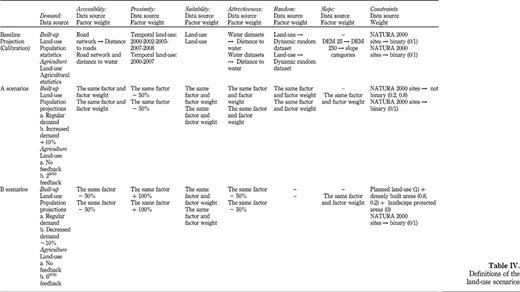
Before the land‐use scenario simulation, calibration procedures were carried out in LUCIA using a combination of its built‐in tools for comparing simulated and historical land‐use changes. During calibration the LUCIA model was run using different factors and factor weights to reproduce changes in the land‐use pattern similar to the observed. The baseline land‐use projection (Table IV) includes the factors and factors weights that together with the stakeholders were identified as optimal to reproduce land‐use changes that took place during the calibration period. In total eight land‐use scenarios representing SRES A2 and B2 for year 2040 were chosen for the nutrient modelling. The scenarios were produced by changing factor weights, by introducing new factors and constraints and to some extent by changing the land‐use demand in respect to the baseline projection as described in Table IV.

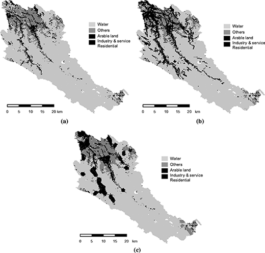
Nutrient modelling was done for the River Temmesjoki river basin (Figure 3). In all land‐use scenarios of year 2040, the river basin will continue to be highly affected by urbanisation due to its vicinity to the growing city of Oulu. The relative share of built‐up area varies between land‐use scenarios. In three decades the total share of the built‐up area will grow from 7 per cent to between 13 and 17.4 per cent. The share of the built‐up area was highest in the A scenario, where the demand for land was increased by 10 per cent and lowest in the B scenario, where the demand was decreased by 10 per cent.

The results from the scenarios with a 10 per cent increase or decrease in urban land demand are not presented in this paper; focus is on the four scenarios, where the demand for built‐up areas is identical. The reason for this is that the changes in demand had such a small effect on the results. For example, at points along the network of Temmesjoki river basin (Figure 2), the impact of using an increased (+10 per cent) or decreased (−10 per cent) demand for the urban classes was marginal, only 0.0‐1.7 per cent, on the P concentrations. In comparison, the feedback mechanism for agriculture has a much bigger impact on the results. It was however useful to make the ±10 per cent runs to find out that the results are not very sensitive to changes in the demand for new urban land. From this point onwards, the chosen scenarios are being referred as A, A+, B, and B+, where the “+” indicates that a feedback mechanism has been used for agriculture.

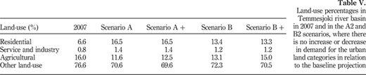
The overall share of agricultural areas is stable in the Oulujoki‐Iijoki RBD as a whole in the scenarios where agricultural feedback has been used. However, in Temmesjoki river basin the share of agricultural areas will decline (Table V). According to the A and B scenarios the agricultural area will decrease from covering 16 per cent in year 2007 to covering 11‐15 per cent in year 2040 depending on the use of a feedback mechanism or not. The share of agricultural areas is the highest in the B+ scenario.

According to the results, it seems most likely that the total amount of the loading of P will decrease at the river basin level (Table VI). Only in the B+ scenario the total loading of P will slightly increase. The main reason for this is that the share of agricultural land‐use is the highest in this scenario.

The total loading figures are very sensitive to the share of agriculture. The overall situation regarding loading would be very different if the total share of agriculture would not decrease in Temmesjoki river basin by the year 2040. During the calibration period, there have emerged comparatively more new built‐up cells than new agricultural cells in Temmesjoki river basin. Since the model extrapolates this trend with small adjustments into the future, the land‐use models have placed proportionally more new agricultural cells elsewhere in the Oulujoki‐Iijoki RBD – in areas of comparatively low demand for urban development.

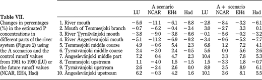
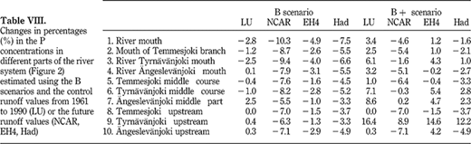
Changes in P concentrations were modelled at different locations along the river system to highlight the differences between the scenarios at a local scale (Figure 2). In general, the concentrations of P seem to decline in the river mouth, but the concentrations may grow inland in points close to the head waters (Tables VII and VIII). This is in line with what is expected regarding the leaching of P, since if the total annual loading remains the same, increased runoff reduces concentration in the river mouth. The extent of the decrease or the increase of P varies depending on the scenario in question. In the points along the river network situated in the head waters (points 5‐10 in Figure 2) the values increase more in the A scenarios. In the B+ scenario the share of agricultural area is the highest, but there is only an increase in P loading in a couple of points at the head waters, due to the emergence of new agricultural cells there. In the B scenario there is no increase what so ever in P loading, when the future hydrological conditions has been taken into account (NCAR, EH4, Had).

The magnitude of the decrease or increase of P concentrations varies depending on the GCM used. When using NCAR the P concentrations decrease the most and increase the least in the points 5‐10 in the head water parts of the rivers (Table VII). When using EH4 values, the biggest increases and the smallest decreases in P loading can be found, while the P concentrations using the Had values seems to be somewhere in between the results from when modelling with NCAR and EH4.

Changes in land‐use itself indicate more increases in P concentrations than if the modelled future runoff is included in the P loading estimations. In the first column (LU) of Tables VII and VIII, only changes in land‐use (LU), and not the GCM climate data have been taken into account. Instead the average runoff for the control period 1961‐1990 has been used. Only in the B2 scenario the loading figures show a decrease at certain points along the river network.

This paper describes an integrated modelling approach for producing regional SRES‐based land‐use scenarios and for integrating them and corresponding climate change variables in nutrient leaching modelling. River basin managers should already be considering how to incorporate the potential effects of climate change into policies and river management plans. Using scenarios, planners and policy makers can be confronted with the outcomes of their decisions or their incapability of making decisions and taking actions (Sohl et al., 2010). Integrated water resource and river basin management could be an instrument to explore adaptation measures to climate change, but so far it is in its starting phase (Kundzewicz et al., 2007). Therefore, it is important to provide examples of approaches, which support the production and use of relevant scenarios.

Access to consistent and sufficiently long time series of land‐use data remains a challenge in land‐use modelling (Sohl et al., 2010). Due to data limitations, the calibration period for the land‐use model was short (seven years) in comparison to the simulated time period (33 years). This is not an ideal situation. It would however, be a more serious problem if the goal was to extrapolate the ongoing development. Since the intention was to base the scenario development on the factors and factor weights identified during the variable and scenario construction process and mainly derive the magnitude of the changes, i.e. the land demand, from the land‐use data, it was not such a serious problem. The basic factors of urban land‐use modelling – suitability, accessibility – are well established and do not require very much validation. The short time span was also compensated for by the access to a consistent time series of built‐up land‐use data – 2000‐2002‐2005‐2007‐2008 – which results in a proximity factor of high quality (Hansen, 2012).

Looking at the results of the nutrient leaching modelling, one can observe that the influence of the agricultural feedback mechanism is large, even as large as the influence of the scenario (Table V). Since P loading is comparatively high from agricultural areas, and the feedback mechanism keeps the overall share of agriculture at a high level, it is only natural and perfectly acceptable that the feedback mechanism has a great impact. From the results, one can also conclude, that the impact of the built‐up structure does not play as big a role. This has to do with the stability of the modelled land‐use scenarios as built‐up areas continue to build upon the historical land‐use structure. Even in the B scenario, where the structure of the urban areas will follow the planned area borders more than they do today, built‐up areas will continue to follow the outlines of the existing settlement structure. The drawback of this stability is that the simulated land‐use scenarios are not very different in the sense of their overall shares of land‐use; the differences lay mainly in the structure and orientation of the new, expanded active land‐use cells.

The results from the nutrient modelling imply that the environmental impact of land‐use and climate change is dependent on the land‐use composition, structure and scale. For example, impacts on river basin level may look very different from the impacts on the local level, at points along the river network. Both scales are of relevance to environmental planners and decision makers dealing with improving the environmental status of water resources. Today many complex hydrological and nutrient leaching models are spatially more or less lumped. But according to this paper and to others (Rankinen et al., 2002) space and spatial structure do matter, implying that geospatial data should be more integrated in nutrient modelling than it is today.

The results also show that the share of agricultural areas plays a central role regarding the leaching and dilution of P in general and along the river network. Where the percentage of agricultural area is high, the overall loading figures are also higher. This is not surprising, since it is generally known that agricultural land is the major source of nutrients (EEA, 2006). However, what is interesting is that differences in the spatial structure of different land‐use classes also seem to have an effect. The land‐use structure can result in a decrease in P leaching even with a comparatively high share of agriculture. This is the case for the B+ scenario having the highest share of agriculture and still its loading figures along the river network are comparatively low. If the spatial land‐use structure can be proved to make a difference, this could have further practical implications for river basin management. However, this finding requires more detailed research. The P leaching results are probably more sensitive at a certain spot than for the study area as a whole and this sensitiveness should be further tested and analysed, before conclusions can be made.

The authors are fully aware of that RLGIS excludes a lot of relevant nutrient processes and that the specific load figures (Table II) upon which the nutrient leaching modelling was based are averages and that real values vary depending on area and on environmental and weather conditions. The specific load figures used, are however the best possible information available and are based on research in Finnish conditions. Despite the use of a simple nutrient leaching model, the overall results are in line with the results of a large European project “climate and lake impacts in Europe” (CLIME). CLIME used the much more complex GWLF model to model the effects of climate change on the supply of P. Like us, they found very little overall change in the annual loading of P at test sites in Europe, of which one was situated in Finland (George, 2010). This indicates that the integrated modelling framework chosen does, despite its simplicity, work.

In this paper, the calculations regarding P loading are based on annual runoff values. Changes in seasonal runoff are likely to be more evident than in annual runoff and the use of seasonal or even daily averages may reveal new aspects regarding P concentrations. The future runoff will also be affected by the future land‐use structure – a fact which has to be addressed in further research. Land‐use scenarios should however also be an integrated part in subsequent research.

This paper suggests an integrated modelling approach for assessing the combined effects of climate change and land‐use change on the leaching of phosphorus at local and regional scale. The cooperation with the stakeholders and the production of region‐specific spatial input variables (datasets) to the land‐use model ensured that regionally relevant SRES‐based land‐use scenarios were produced.

The results of the nutrient modelling imply that the modelling framework works, as they are in line with the results of others (George, 2010). The individual models and model components are not new or totally comprehensive, but instead transparent and easy to understand also for decision makers and environmental planners, which clearly is a benefit for its possible use in practice.

Many of the present nutrient leaching models does not include a spatial component. The results however suggest that including a spatial component in nutrient modelling should be considered: the results of this paper imply that the environmental impact of land‐use and climate change is dependent on the land‐use composition, structure and scale, and not only on shares of the land‐use categories. Environmental planners could use the modelling framework to discuss region‐specific development options with decision makers and land‐use planners, and to show that not only the share of agriculture plays a role when it comes to the problem of nutrient leaching. To reach the goal to achieve a good water quality in a river basin, also the spatial land‐use structure may play a role. Further research on the findings of this paper is needed in order to fully understand how the spatial land‐use structure affects water quality on a general level and in order to make guidelines on how this can be used in practice in river basin and other water management.

The current work was carried out as part of the WaterPraxis project (www.waterpraxis.net). This project was co‐financed by the Baltic Sea Region Programme under the Regional Development Fund of the European Union. The authors would like to thank the anonymous reviewers for their valuable comments for improving this manuscript.

Lena Hallin‐Pihlatie (MSc) has a degree in physical geography from Helsinki University. She works as a GIS expert at the Finnish Environment Institute. Her main work is related to land‐use planning and modelling, land monitoring and the implementation of the INSPIRE Directive. She is involved in national and international projects related to land cover, land use, water management and climate change. Lena Hallin‐Pihlatie is the corresponding author and can be contacted at: lena.hallin‐pihlatie@environment.fi

Jaana Rintala (MSc) has a degree in biophysics from Oulu University, Finland. She works as an environmental planner at the Centre for Economic Development, Transport and the Environment for North Ostrobothnia. Her expertise is in GIS‐based modelling and she works with national and international projects related to river basin management.

Henning Sten Hansen is Professor in Geoinformatics at Aalborg University, Copenhagen. He has been working in the field of geoinformatics and environmental geography for more than 20 years. His main research fields are geospatial modelling, land use, climate change management, and infrastructure for spatial information. He is a member of the Editorial Board of the International Journal of Climate Change Strategies and Management, and the Executive Committee of the European Umbrella Organisation of Geographic Information (EUROGI).