


Major shifts in the southern hemisphere circulation occurred during the mid‐1970s concurrent with large reductions in southern Australian winter rainfall associated with decreased cyclogenesis. The purpose of this paper is to study changes in cyclogenesis over southern Australia during the last 50 years, examine the ability of coupled climate models to simulate the winter circulation changes, and discuss projected changes in winter circulation and rainfall under different climate change scenarios.
Three dimensional instability theory is used to study changes in cyclogenesis. The response of 22 coupled model intercomparison project three (CMIP3) IPCC climate models to observed increases in greenhouse gases, from pre‐industrial to the end of the twentieth century, is examined. The authors focus on two diagnostics closely related to the changes in cyclogenesis: changes in the 300 hPa zonal wind strength; and changes in the baroclinic instability. Projected changes in baroclinic instability and rainfall are investigated in SRESB1, SRESA1B and SRESA2 scenarios.
There has been a 30 per cent reduction in the growth rate of the leading storm track mode crossing southern Australia in the 1975‐1994 period, and a 37 per cent reduction in the 1997‐2006 period, when compared to 1949‐1968. Most of the CMIP3 models capture the changes in the zonal wind; only about a third the changes in baroclinic instability. Projected changes in baroclinic instability and rainfall suggest further reductions in the growth rate of storm track modes and further large reductions in rainfall over southern Australia.
The paper addresses a major cause of the reduction in Australian winter rainfall, and provides guidance on future‐projected changes.
1. Introduction
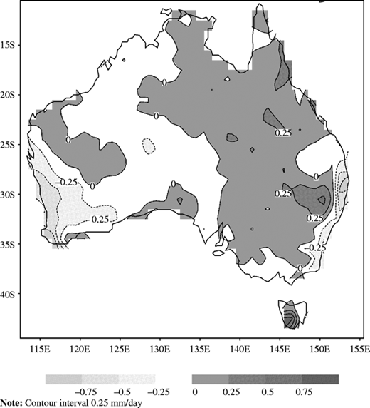
The early to mid‐1970s was a time of major shifts in the structure of the large‐scale circulation of both the northern and southern hemispheres (SHs) (see Frederiksen and Frederiksen (2005, 2007), for overview). Over southern Australia there was a concurrent, dramatic and continuing reduction in the winter rainfall with very large reductions (∼20 per cent) occurring first in the southwest of Western Australia (SWWA) (Sadler et al., 1988; Allan and Haylock, 1992; Hope et al., 2006; Nicholls, 2007; Bates et al., 2008; Ummenhofer et al., 2008). For example, Figure 1 shows differences in Australian July rainfall between 20‐year averages over the periods 1949‐1968 and 1975‐1994, using the Australian Bureau of Meteorology National Climate Centre high quality‐gridded dataset. This shows large reductions over SWWA and eastern‐southeastern Australia, amounting to reductions of around 20, 30 and 10 per cent, respectively. Since then there has been a continuing decline in the southwest and during the last decade or so, large reductions in the southeast (Cai and Cowan, 2008).
In trying to explain this reduction in SWWA, Frederiksen and Frederiksen (2005, 2007) studied the interdecadal changes in SH winter cyclogenesis by focusing on the leading instability modes for three‐dimensional basic states averaged over the periods 1949‐1968 and 1975‐1994 for the month of July, as well as other shorter periods, using reanalyzed National Centres for Environmental Prediction (NCEP) (Kalnay et al., 1996) and the European Centre for Medium Range Weather Forecasting Reanalysis (ERA40) (Uppala et al., 2005) data. They found that there was a 30 per cent reduction in the growth rate of the cyclogenesis modes in the latter period compared with the earlier. In addition, the leading mode in each period has a different three‐dimensional structure. For the 1949‐1968 basic state, the leading mode is a wavenumber 12 disturbance with large amplitude over southern Australia (Figure 7); for the 1975‐1994 basic state the leading SH cyclogenesis mode is a wavenumber 8 disturbance with maximum amplitude in the central South Pacific ocean, and only small amplitude south of southern Australia (Figure 8). However, they did find similar subdominant modes with a similar structure and frequency, but reduced growth rate (∼30 per cent).
Frederiksen and Frederiksen (2005, 2007) suggested that these differences could be explained in terms of the differences in the mean climate of the two periods. In particular, the reduction in the vertical wind shear, or baroclinicity, in the region of the subtropical jet stream, and associated with dramatic reductions in the jet strength, was shown to be largely responsible for the reduction in growth rate. Their results were also insensitive to the reanalysis dataset used, suggesting that they are fairly robust. They concluded that a primary cause of the rainfall reduction over SWWA, and southern Australia generally, was due to these changes in the cyclogenesis modes that affect this region. In addition, these changes in baroclinicity were shown to be hemispheric in extent in a band near 30S, suggesting associated hemispheric‐wide reductions in rainfall.
Here, we examine the extent to which comprehensive coupled ocean‐atmosphere climate models show similar atmospheric winter circulation changes, as seen in Frederiksen and Frederiksen (2005, 2007) for the reanalysis datasets. In particular, we consider the response of the Coupled Model Intercomparison Project Three (CMIP3) climate models (Meehl et al., 2007) to observed natural and anthropogenic forcing, including increasing greenhouse gases, from pre‐industrial to the end of the twentieth century. We also look at the projected changes in SH baroclinicity and rainfall for each of the three Special Report on Emission Scenarios (SRES) B1, A1B and A2 (Meehl et al., 2007) and the impact on water resources over southern Australia in particular.
The plan of this paper is as follows. In Section 2, we give a brief overview of the changes in the SH winter cyclogenesis, or storm track, modes from reanalysis data during the last 50 or so years, concentrating on those that affect southern Australia. In Section 3, we discuss those changes in the climate of the winter SH circulation that are largely responsible for the changes in SH cyclogenesis. We also consider the ability of the CMIP3 models to reproduce these changes. In Section 4, we look at projected changes in SH winter baroclinic instability and rainfall in the SRESB1, SRESA1B and SRESA2 scenarios. Our conclusions are in Section 5.
2 Changes in SH winter cyclogenesis
The generational mechanisms and dynamical properties of SH synoptic scale cyclogenesis have been successfully described with three dimensional instability theory (Frederiksen and Frederiksen, 1993) using primitive equation atmospheric models linearised about a basic state climate. Here, we have used the primitive equation instability model described in Frederiksen and Frederiksen (1992, 2005, 2007) to highlight the changes that have occurred in the growth rate and structure of the storm track modes that affect southern Australia.
The current version of the model includes a generalized Kuo‐type heating parameterization that incorporates closures for both convection and evaporation‐wind feedback as described by Frederiksen (2002). Each of the perturbation fields and basic state fields, entering the linearised equations, is expanded in terms of spherical harmonics with the perturbations also having time dependence exp(−iωt). Here, t is the time and ω=ωr+iωi is the complex angular frequency with ωr being the frequency and ωi the growth rate. This then results in a system of eigenvalue‐eigenvector equations described in Frederiksen and Frederiksen (1992) for the perturbation field variables of stream function, potential temperature and velocity potential. A so‐called rhomboidal 15 truncation is used for both the perturbation and basic state fields in which the zonal wavenumber m=−15, … , 0, … , 15 and the total wavenumber n=|m|, |m|+1, … , |m|+15 in the spherical harmonic expansion. In this study, we use typical parameters for the strength of the convection, evaporation and dissipation as described in Frederiksen and Frederiksen (2005). A review of instability theory and applications is given by Frederiksen (2007).
We concentrate on the three periods 1949‐1968, 1975‐1994 and 1997‐2006. Also, because our main concern here is with the impact of the circulation changes on rainfall, we present the results in terms of the upper level divergence field of the cyclogenesis modes. Frederiksen and Frederiksen (2007) show that precipitation, due to convection is proportional to the upper level divergence in their model. Thus, Figure 2(a) shows the divergence of the fastest growing instability mode (mode 1) for the period 1949‐1968. It is a SH cyclogenesis mode consisting of a series of eastward propagating troughs and ridges with largest root mean square divergence amplitude (Figure 2(b)) over SWWA. That is, it has maximum impact on rainfall over this region. Figure 2(b) also defines the storm track associated with this mode. The periodicity of this mode is about 1.2 days and the growth rate is 0.423 day−1.
In the period 1975‐1994, the fastest growing SH cyclogenesis mode (mode 8) has a different horizontal structure with maximum divergence amplitude in the central South Pacific, very little influence over southern Australia (not shown). However, mode 9 (Figure 2(c)) has a very similar structure (Table I) and periodicity to mode 1 in the earlier period. Its growth rate is 33.5 per cent lower (Table I), consistent with the observed reduction in rainfall over southern Australia, and in particular SWWA. In fact, the growth rates of the ten leading cyclogenesis modes, crossing Australia in this period, have been reduced by 33 per cent or more when compared with similar modes in the earlier period. Figure 2(d) shows the corresponding cyclogenesis mode (mode 12) for the more recent period 1997‐2006. The growth rate of this mode has continued to decline by 37 per cent when compared with the 1949‐1968 period (Table I). Again, this reduction of the growth rate is true for all the ten fastest growing cyclogenesis modes crossing southern Australia in the later periods.
3. Changes in the SH wintertime circulation and rainfall
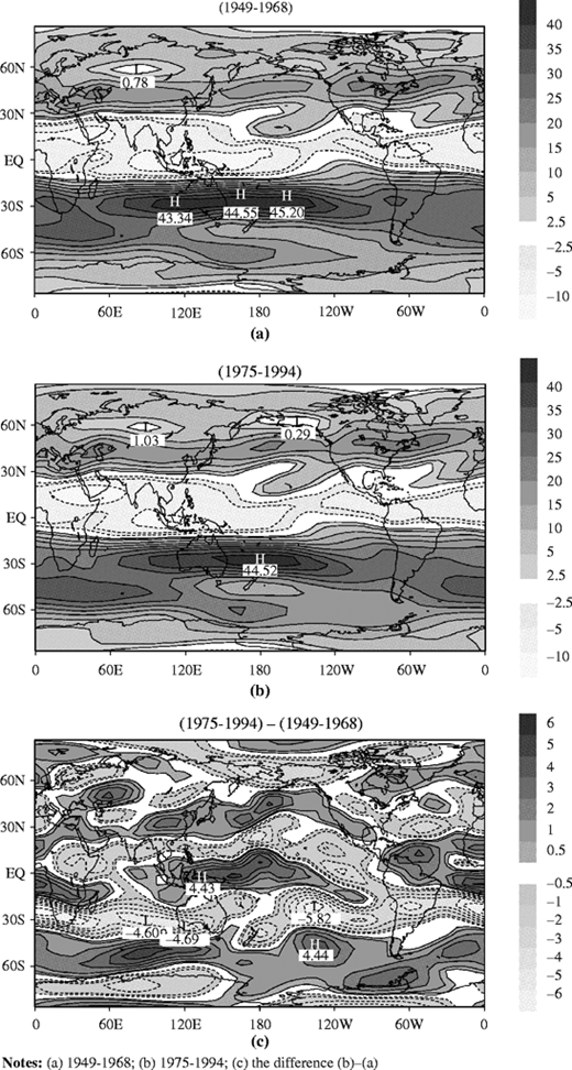
Frederiksen and Frederiksen (2007) found that there were quite large changes in the thermal structure and circulation in the SH circulation between the periods 1949‐1968 and 1975‐1994. In particular, there was reduction (17 per cent) in the strength of the subtropical 300 hPa zonal wind upstream and over southern Australia, and extending over much of the hemisphere. Near 45‐50°S, there was an increase in zonal wind. Also, they found a reduction in the baroclinic instability, as measured by a generalization of the Phillips (1954) criterion (see below), of between 25 and 30 per cent upstream and over SWWA. Because our interest here is on changes in the atmospheric circulation that affect cyclogenesis, these are two good diagnostics to use to evaluate the climate models. They are also very much related to other changes discussed by Frederiksen and Frederiksen (2007), including a reduction in the mean atmospheric meridional temperature gradient, changes in the Hadley circulation, and trends in the Southern Annular Mode. Here, we will compare the model results with the NCEP reanalysis.
3.1. Changes in 300 hPa zonal winds
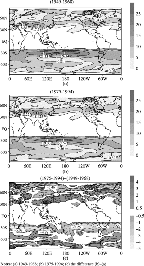
Figure 3 shows the NCEP 300 hPa zonal velocity averaged over the periods 1949‐1968 and 1975‐1994, and their differences. The difference plot (Figure 3(c)) shows quite dramatic reductions near 30°S in the latter period of up to 7 ms−1, and increases between 5 and 6 ms−1 further south near 50°S. These differences in the zonal wind structure are clearly hemispheric and unlikely to be the response to some local phenomenon. Of particular interest is the region 60‐150°E, 60‐15°S. Frederiksen and Frederiksen (2007) showed that this area is very much related to the genesis of the storms that affect southern Australia. In this area, there are reductions in the sub‐tropical zonal velocity of up to 4.7 ms−1 with increases up to 5.6 ms−1 further south.
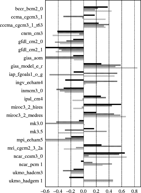
In Figure 4, we show the anomaly pattern correlation (APC), calculated over the domain (60‐15°S, 60‐150°E) between the NCEP difference in 300 hPa zonal winds (Figure 3(c)) and similar differences for 22 of the CMIP3 models (see Randall et al. (2007) and Meehl et al. (2007), for model nomenclature and description). The model differences were calculated in four different ways. The black bars in Figure 4 are the APCs with zonal wind differences calculated for models using the same two 20‐year periods 1949‐1968 and 1975‐1994 as for the NCEP reanalysis (i.e. the 20C3M simulations; Meehl et al., 2007). However, because the timing of the simulated changes in coupled models may not necessarily synchronize with the reanalyzed observations, we have also included APCs with model differences between pre‐industrial control runs (i.e. the PICNTRL simulations; Meehl et al. (2007)) and the 1980‐1999 period of the 20C3M runs. This will give an indication of the impact of all the twentieth century greenhouse gas forcing. Also, we are interested in the sensitivity of our results to the base period chosen in the PICNTRL runs, and the possible influence of decadal variability on our results. For this reason, we have used three adjoining 20‐year periods at the end of the PICNTRL runs, separated by 20 years. These are designated PICNTRL (dark shading), PICNTRL_20 (medium shading) and PICNTRL_40 (light shading).
Figure 4 shows that the ability of the models to reproduce the reanalysis changes during the same two 20‐year periods is quite variable, with some models showing opposite sign in the zonal wind differences. When changes from pre‐industrial simulations are taken into account, there is clear evidence of a component of decadal variability with the APCs showing some dependence on the base period. For some models, this is seen in the changing sign of the APC (e.g. gfdl_cm2_1), and for others in changes in the magnitude of the APC (e.g. mk3.0). Some models show quite large APC with the reanalysis results (e.g. miroc3_2_medres, miroc3_2_hires and giss_model_e_r). A number of models show consistently positive APC in all four cases (e.g. miroc3_2_medres, miroc3_2_hires and mk3.0). Overall, the majority of the models do simulate the direction of the changes in the zonal wind upstream and over southern Australia, especially in differences between the pre‐industrial and end of the twentieth century simulations, but the changes are generally smaller than observed.
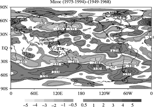
The miroc3_2_medres, in particular, simulates the SH changes seen in Figure 3(c) remarkably well (Figure 5). The model captures the hemispheric nature of the differences with negative anomalies near 30°S, and positive anomalies near 50°S. The reduction in the zonal wind upstream and over southwestern Australia is well simulated, as is the increase further south, although the differences are generally smaller than in the reanalysis data.
3.2. Changes in baroclinic instability
A simple diagnostic that provides a measure of incipient baroclinic instability is the Phillips (1954) criterion. It can be used to identify geographical regions of likely cyclogenesis (Frederiksen and Frederiksen, 1992). This criterion may be written, generalized for spherical geometry, as: Equation 1 where u¯(1) and u¯(3)represent the 300 and 700 hPa zonal velocities, and σ¯ the static stability for a given basic state, calculated here as half the difference between the potential temperature at 300 and 700 hPa. Here, cp=1, 004 J°−1 kg−1, is the specific heat of air at constant pressure, Ω=7.292×10⁻⁵ rad s−1, is the earth's angular speed of rotation, bκ=0.124 is a dimensionless constant, a=6.371×10⁶ m, is the radius of the earth and ϕ is latitude. The criterion is always negative near the equator, and is, therefore, mostly relevant for the development of extra‐tropical cyclogenesis.
In Figure 6, we show regions where this baroclinic instability criterion is positive for the NCEP reanalysis 1949‐1968 and 1975‐1994 basic states, and their difference, respectively. In July, these regions coincide with the sub‐tropical jet and a maximum in the criterion occurs in the South Pacific near 30°S. There are quite large reductions (4‐5 ms−1) in the criterion in the latter period that extends across the whole hemisphere in a band centred near 30°S (Figure 6(c)). Frederiksen and Frederiksen (2007) show that this is associated with a reduction of cyclogenesis throughout this band and the reduction in growth rate of the SH climatological cyclogenesis modes. This is consistent with the results shown in Figure 2 and Table I. In other words, the SH has essentially become less baroclinically unstable near 30°S in the latter period compared with the former. In contrast, poleward of about 45°S there is an increase in baroclinic instability, especially south and upstream of Australia. Importantly, there are reductions upstream and across southern Australia consistent with a reduction in growth rate of storm modes and reduced rainfall. Over SWWA there is a reduction of about 4.5 ms−1.
Figure 7 shows the APCs, calculated for the region 60‐150°E, 45‐15°S, between the NCEP Phillips criterion difference (Figure 6(c)) and the model differences for the same four cases discussed in the previous section. For this diagnostic, there is much more variability in the models to simulate the reanalysis results. About a third of the models show a consistently negative APC, in all four cases (e.g. gfdl_cm2_1, giss_aom, mpi_echam5, etc.). For these models, there is an increase in baroclinic instability that would lead to an increase in growth of the cyclogenesis modes. However, about a third of the models show a consistently positive APC (e.g. miroc3_2_medres, giss_model_e_r, ncar_ccsm3_0, etc.). Again, as for the zonal velocity, there is evidence of a component of decadal variability in the model results.
With respect to the two diagnostics we have considered, the miroc3_2_medres model agrees fairly consistently with the NCEP reanalysis changes (Figures 4 and 7) but of smaller magnitude. This is clear from Figure 5, for the zonal wind differences, and Figure 8 which shows the Phillips criterion differences for this model in all four cases. The difference between the 1980‐1999 period and the last 20 years of the PICNTRL run is remarkably similar to the NCEP changes (Figure 6(c)) throughout the subtropical SH. The changes in baroclinic instability upstream of Australia are fairly consistent in all cases, and matches the NCEP changes, suggesting that this is a robust result for this model.
3.3. Changes in rainfall
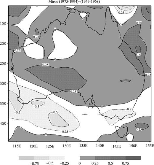
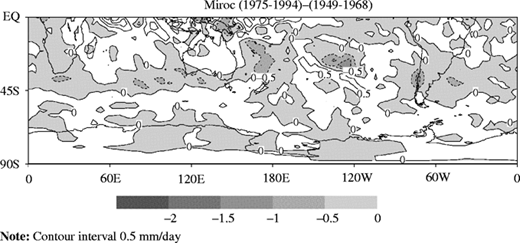
For the remaining part of this paper, we are going to concentrate on the results from the miroc3_2_medres model. This model shows reductions in rainfall over SWWA and southeastern Australia, in particular, which are consistent with the observations for the periods 1949‐1968 and 1975‐1994, although underestimated. This can be seen from Figure 9, which shows reductions over SWWA up to 0.5 mm/day (compared with 0.8 mm/day in Figure 1) and up to 0.4 mm/day or more over southeastern Australia (compared with about 0.2 mm/day in Figure 1). Figure 10 shows that there are also reductions in rainfall in a hemispheric band around 30°S consistent with the reduction in baroclinic instability (Figures 6 and 8). Further south there are increases in precipitation coinciding with increases in zonal wind and baroclinicity. Qualitatively similar changes in rainfall are also seen in the other models that capture the changes in both the zonal wind and Phillips criterion (for example, the giss_model_e_r and ncar_ccsm3_0 models).
4. Projected changes in baroclinic instability and rainfall
The CMIP3 models, considered here, were all used in a series of climate change scenarios. Here, we will consider three such scenarios; the SRES B1, A1B and A2 (Meehl et al., 2007). These involve low, medium and high CO2 concentrations of 550, 700 and 820 ppm, respectively, by 2,100. We will focus on projections of possible changes in baroclinic instability and rainfall using the miroc3_2_medres model.
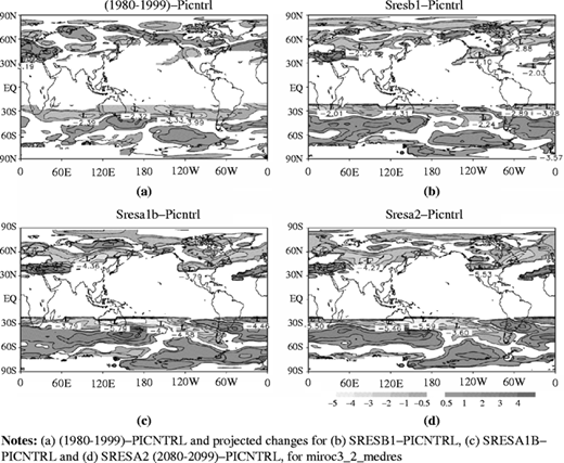
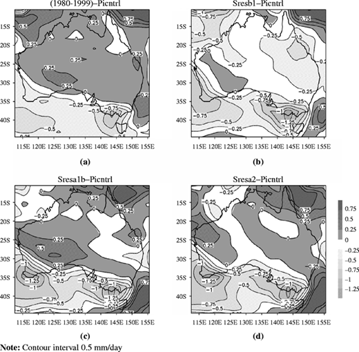
In Figure 11, we show the changes in Phillips criterion for 1980‐1999 – PICNTRL, SRESB1‐PICNTRL, SRESA1B‐PICNTRL and SRESA2‐PICNTRL, using this model. For each of the SRES scenarios we have used the 20‐year period 2080‐2099 for comparison. As the CO2 concentrations increase beyond present day values, there are in all three SRES cases much larger reductions in the subtropical baroclinic instability when compared with the 1980‐1999‐PICNTRL differences, especially over southern Australia. For SRESB1, peak reductions are about double those seen in 1980‐1999. The largest reductions occur for SRESA1B and SRESA2, showing the increasing impact of the much larger CO2 concentrations. Because the Phillips criterion is a measure of incipient baroclinic instability, these results suggest that there would be further reductions in the growth rate of the SH storm track modes, especially for those impacting on southern Australia. This would imply further reductions in winter rainfall and worsening drought conditions over southern Australia. The increase in baroclinic instability further south implies increase cyclogenesis on the polar jet together with the possibility of increased rainfall.
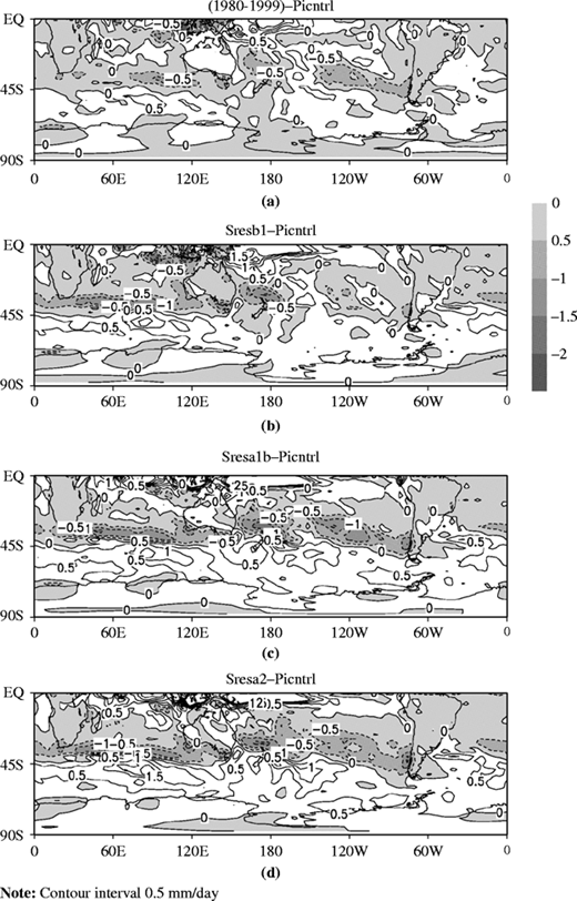
This is indeed the case for the miroc3_2_medres model, when we consider the corresponding changes in rainfall for these scenarios. Figure 12 shows the rainfall differences for the present day and each scenario compared to the PICNTRL rainfall. In each case, there are reductions over southern Australia and in a hemispheric band centred near 30°S, and increases further south. For 1980‐1999, rainfall reductions, in this band, range between 0.5 and 1.0 mm/day. Further south there are increases peaking around 0.5 mm/day. Over Australia (Figure 13) peak reductions approaching 0.5 and 0.75 mm/day occur in the far southwest and southeast, respectively. Under the SRESB1 scenario, there are further reductions with some values less than −1.5 mm/day. Significant parts of the southwestern Australia have reductions over 0.75 mm/day and in the southeast reductions just exceed 1.0 mm/day. There are also larger increases near 45°S exceeding 1 mm/day. This trend continues for increasing CO2 concentrations (SRESA1B and SRESA2), with reductions approaching 1.5 mm/day over wide spread areas of the subtropical band. Over Australia, there are peak reductions of more than 1.25 mm/day in the southwest and southeast. Near 45°S, there are increases in excess of 1.5 mm/day.
Qualitatively similar results are also seen from the models that reproduced the twentieth century changes in our two diagnostics (e.g. the giss_model_e_r, miroc3_2_hires and ncar_ccsm3_0 models).
5. Conclusions
There have been large reductions in winter rainfall over southern Australia since the mid‐1970s. A comparison of the average rainfall over the 20‐year periods 1949‐1968 and 1975‐1994, shows that the largest reductions have occurred in the southwest, southeast and east coast. There has been a further decline to the present day. Here, we have considered the changes in the growth rate and structure of the storm track modes that affect southern Australia, using as July basic states the large‐scale circulation and thermal structure for the periods 1949‐1968, 1975‐1994 and 1997‐2006. These periods are distinguished, in particular, by a worsening decline in the peak of the July jet stream and significant reductions in the subtropical baroclinic instability as measured by the Phillips criterion. As a result, there has been a 30 per cent reduction in the growth rate of the leading storm track mode crossing southern Australia in the 1975‐1994 period, and a 37 per cent reduction in the 1997‐2006 period, when compared to 1949‐1968. This is a primary cause of rainfall reduction over southern Australia, and throughout the subtropical hemisphere, in winter.
In this paper, we have investigated the ability of the CMIP3 models to simulate the changes in two important diagnostics related to the growth of storm track modes. These are the changes in the climatological SH upper level zonal wind and the Phillips criterion for incipient instability between the periods 1949‐1968 and 1975‐1994. Both of these diagnostics show large reductions in a subtropical band, and increases further south near 45°S. These changes directly influence the changes in the storm track modes. Most of the 22 CMIP3 models capture the changes in the zonal wind, but only about a third reproduce the changes in the baroclinic instability condition. The models generally best reproduce the changes when the total CO2 concentration increase from pre‐industrial conditions is used. It is clear from the results presented here that there is a component of decadal variability in the model results that is dependent on the base period chosen in the pre‐industrial runs. This means that attribution and projection of atmospheric circulation changes may involve the disentanglement of decadal variability and anthropogenic climate change.
We have also considered the impact of further increases in CO2 concentrations using the SRESB1, SRESA1B and SRESA2 scenarios. There are a number of models that consistently, in all the four cases considered here, simulate changes in the zonal wind and Phillips criterion similar to those seen in the NCEP reanalysis. Projected changes in baroclinic instability from these models suggest that further large reductions, between two and two and a half times, in baroclinic instability are possible in the subtropics under SRESB1, SRESA1B and SRESA2 scenarios, especially over the Australian region. These models also show further reductions in rainfall over southern Australia, and in a subtropical band throughout the hemisphere and consistent with areas that show reductions in baroclinic instability. Reductions from the pre‐industrial over the southwest and southeast of Australia can be as much as twice those seen at the end of the twentieth century.
Importantly, this study shows that the changes in circulation and rainfall during the twentieth century can be reproduced in a number of models forced by the observed increasing greenhouse gases. When forced by further increases in greenhouse gases, as in the SRES scenarios, the same structure of changes occur, but with larger magnitude.
The results presented here suggest the possibility of further large reductions in rainfall over southern Australia during this century. This has important ramifications for future planning and management of the water supply, agriculture, food supply and sustainable population projections for Australia.

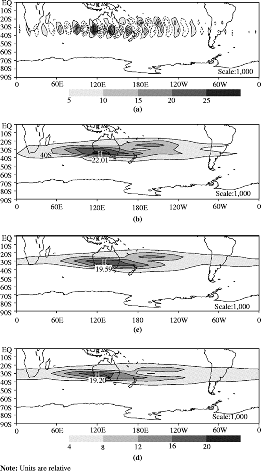
(a) The divergence of July storm mode 1, for the period 1949‐1968; (b)‐(d) the divergence amplitude for modes 1, 9 and 12 for the periods 1949‐1968, 1975‐1994 and 1997‐2006, respectively
(a) The divergence of July storm mode 1, for the period 1949‐1968; (b)‐(d) the divergence amplitude for modes 1, 9 and 12 for the periods 1949‐1968, 1975‐1994 and 1997‐2006, respectively
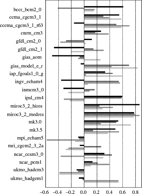
APC between the NCEP 300 hPa zonal velocity difference (Figure 1(c)) and model difference for (1975‐1994)−(1949‐1968) (black bar); (1980‐1999)−PICNTRL (dark shade); (1980‐1999)−PICNTRL_20 (medium shade); (1980‐1999)− PICNTRL_40 (light shade)
APC between the NCEP 300 hPa zonal velocity difference (Figure 1(c)) and model difference for (1975‐1994)−(1949‐1968) (black bar); (1980‐1999)−PICNTRL (dark shade); (1980‐1999)−PICNTRL_20 (medium shade); (1980‐1999)− PICNTRL_40 (light shade)
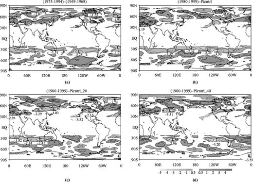
Differences in Phillips criterion (ms−1) for (a) (1975‐1994)− (1949‐1968), (b) (1980‐1999) − PICNTRL, (c) (1980‐1999)−PICNTRL_20 and (d) (1980‐1999) PICNTRL_40, for miroc3_2_medres
Differences in Phillips criterion (ms−1) for (a) (1975‐1994)− (1949‐1968), (b) (1980‐1999) − PICNTRL, (c) (1980‐1999)−PICNTRL_20 and (d) (1980‐1999) PICNTRL_40, for miroc3_2_medres

This research is partly supported by the West Australian Department of Environment and Conservation under the Indian Ocean Climate Initiative Stage 3 and the Australian Climate Change Science Program of the Australian Department of Climate Change. The authors acknowledge the modeling groups, the Program for Climate Model Diagnosis and Intercomparison and the World Climate Research Program's Working Group on Coupled Modeling for their roles in making available the CMIP3 multi‐model dataset.
References
About the authors
Carsten Segerlund Frederiksen is a Senior Principal Research Scientist at the Australian Bureau of Meteorology and Team Leader of the Climate Processes team within the Centre for Australian Weather and Climate Research. He has a PhD in Computational Fluid Dynamics. His research interests cover climate change and attribution studies and causes, climate variability and predictability and dynamical and statistical seasonal prediction, especially with respect to Australian climate. His expertise includes dynamical theories of atmospheric processes and mechanisms for the development of atmospheric disturbances ranging from cyclogenesis, blocking, intraseasonal oscillations, monsoon disturbances and large‐scale teleconnections. He has also helped develop theories and statistical methods for identifying modes of inter‐annual variability of seasonal mean climate data related to slow (predictable) and chaotic processes. Carsten Segerlund Frederiksen is the corresponding author and can be contacted at: c.frederiksen@bim.gov.au
Jorgen Segerlund Frederiksen is a Chief Research Scientist at CSIRO Marine and Atmospheric Research and Fellow of the Australian Academy of Science. He has a PhD in Theoretical Physics and a DSc in Atmospheric Physics. His research interests include dynamical theories of atmospheric processes including storm tracks, blocking, teleconnection patterns, intraseasonal oscillations, monsoon disturbances and equatorial waves; weather prediction and seasonal climate prediction; regime transitions in complex systems such as the atmosphere and coupled ocean atmosphere system; statistical theories of climate states and coherent atmospheric modes; closure theories of turbulence interacting with large‐scale flows, Rossby waves and topography; parameterisations of small scale dynamical processes that improve simulations of atmospheric and oceanic circulations and climate; and causes of Australian climate change during the twentieth century and the likely projected changes in future.
Janice Maria Sisson is a Senior Information Technology (IT) Officer with the Bureau of Meteorology, supplying scientific and IT support, including diagnostic analysis, to projects on climate variability and change with reference to the atmospheric circulation and Australian climate, as well supporting projects on dynamical and statistical seasonal prediction. This author provides IT knowledge and management in accessing and extracting archived data and variables and in running jobs and models (climate models, simple atmospheric models) on supercomputers and linux clusters with mass‐store archive.
Stacey Lee Osbrough joined CSIRO Marine and Atmospheric Research division four years ago with a background in Computer Science and Space Science. Her current role as a Support Scientist is to provide skills in programming and data analysis for the Climate Processes team, a collaboration of people from the Australian Bureau of Meteorolgy and CSIRO. Stacey's work involves investigating ensemble prediction methods using a primitive equation model run on a high‐performance super computer and managing large data sets created by IPCC climate models. She examines this output by employing statistical and data visualisation software to aid further research on future climate change scenarios.

