


Recent advances in hydrological impact studies point that the response of specific catchments to climate change scenario using a single model approach is questionable. This study was aimed at investigating the impact of climate change on three river basins in China, Ethiopia and Norway using WASMOD and HBV hydrological models.
First, hydrological models' parameters were determined using current hydro‐climatic data inputs. Second, the historical time series of climatic data was adjusted according to the climate change scenarios. Third, the hydrological characteristics of the catchments under the adjusted climatic conditions were simulated using the calibrated hydrological models. Finally, comparisons of the model simulations of the current and possible future hydrological characteristics were performed. Responses were evaluated in terms of runoff, actual evapotranspiration and soil moisture change for incremental precipitation and temperature change scenarios.
From the results obtained, it can be inferred that two equally well calibrated models gave different hydrological response to hypothetical climatic scenarios. The authors' findings support the concern that climate change analysis using lumped hydrological models may lead to unreliable conclusions.
Extrapolation of driving forces (temperature and precipitation) beyond the range of parameter calibration yields unreliable response. It is beyond the scope of this study to reduce this model ambiguity, but reduction of uncertainty is a challenge for further research.
The research was conducted based on the primary time series data using the existing two hydrological models to test the magnitude differences one can expect when using different hydrological models to simulate hydrological response of climate changes in different climate zones.
Introduction
Climate change may cause significant impacts on water resources by resulting changes in the hydrological cycle. Increasing temperature will lead to greater amounts of water vapour in the atmosphere and the hydrological cycle will be intensified with more precipitation. However, the extra precipitation will not be equally distributed around the globe. Some parts of the world may see significant reductions in precipitation, or alterations in the timing of wet and dry seasons and would lead to increases in both floods and droughts (Seino et al., 1998; Walsh et al., 2012; Parry et al., 2012; Zhang et al., 2012). The spatial change in amount, intensity, and frequency of the precipitation will affect the magnitude and frequency of river flows; consequently, it will substantially affect the water resources at local and regional levels.
Quantitative estimates of the hydrological effects of climate change at local and regional scales are essential for understanding and solving the potential water resource management problems associated with water supply for domestic and industrial water use, power generation, and agriculture (Steele‐Dunne et al., 2008; Chen et al., 2012a). Therefore, the ability to understand the hydrologic response of climate change will help policy makers to guide planning and form more resilient infrastructure in the future.
Hydrological models provide a framework to conceptualise and investigate the relationships between climate, and water resources (Xu, 1999; Jothityangkoon et al., 2001; Xu et al., 2005; Chen et al., 2012b; Jung et al., 2012; Jiang et al., 2012; Yang et al., 2012). A number of studies have investigated hydrological impact of climate change in different regions (Xu, 2000; Christensen et al., 2004; Jha et al., 2006; Beldring et al., 2008; Steele‐Dunne et al., 2008; Graham and Jacob, 2000; Engeland et al., 2001). Jiang et al. (2012) employ comparison of hydrological impact of climate change using six hydrological models in Dongjiang basin and the result showed that significant differences exist in the predicted runoff, actual evapotranspiration and soil moisture between hydrological models. The key differences between the study presented here and those studies are the use of two hydrological models rather than single hydrological models and testing the magnitude difference in three different climate zones. The two models used to investigate the hydrological impact of climate change are HBV‐light, daily water balance model described in Seibert (1998) and Water And Snow balance MODeling system (WASMOD), monthly water balance model described in Xu (2002) and Xu et al. (1996). Another issue with modeling hydrological impact of climate change is how to capture the full range of climate change scenarios. A number of different methods exist to construct climate change scenarios that include techniques utilising climate analogues, synthetic scenarios, and general circulation model (GCM) scenarios (Carter et al., 1995). In this study, with the goal of testing the magnitude difference of hydrological model prediction in different climate zones, hypothesized scenarios are applied. Given the differences of approaches and downscaling techniques, the use of hypothesized scenarios as input to catchment‐scale hydrological models is widely used (Xu, 2000; Graham and Jacob, 2000; Engeland et al., 2001; Boorman and Sefton, 1997). The main objective of this study is to test the magnitude differences one can expect when using different hydrological models in different regions to predict hydrological impact of climate change.
Materials and methods
Study areas and data
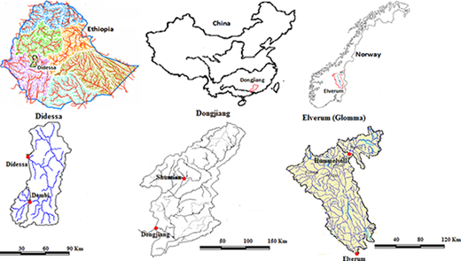
The study was conducted on three river basins in three continents representing a range of geographic and climatic conditions (Figure 1):
(1) Dongjiang river basin: is one of the Zhujiang sub‐basins located in Guangdong and Jiangxi provinces in Southern China. The drainage area of the river basin is 25,555 km2 and flows from north‐east to south‐west direction. For this study, areal rainfall was calculated from the records of the 51 stations using the Thiessen polygon method, mean daily temperature from eight stations and evaporation data from five stations were organized in order to use as model input for the period of 1978‐1988.
(2) Didessa river basin: is located in the South Western part of Ethiopia. The catchment area encompasses approximately 9,981 km2 up to the river gauge near Arjo. Didessa river is a part of the Upper Blue Nile drainage system and it covers around 5.4 percent of the Upper Blue Nile basin area and the river is the largest tributary of Upper Blue Nile river which contributes 10.7 percent of the total discharge (Conway, 2000).
For this study, areal rainfall records were calculated using the Thiessen polygon method from ten rainfall stations for the period from 1985 to 1999:
(3) Elverum basin: is a part of Glomma basin and located in the South Eastern part of Norway.
The drainage area of the basin up to Elverum river gauge station is 15,449 km2. The hydrology of the area is characterized by low flow during winter caused by snow accumulation and high flow during snow melt in spring or early summer (Henny et al., 2008). All the hydro‐climatic data were acquired from Norwegian Water Resource and Energy Directorate (NVE) and Norwegian Meteorological Institute (eKlima).
In order to evaluate the models' performance at different catchment scales, small nested catchments of Shuntian, Dembi, and Hummelvoll which are found within Dongjiang, Didessa, and Elverum basins, respectively, were also examined.
Approach
The study follows four steps (Xu, 1999; Xu et al., 2005):
- 1.
the parameters of hydrological models were determined in the study basins using current climatic inputs and observed river flows from model calibration;
- 2.
the historical time series of climatic data were adjusted according to the climate change scenarios;
- 3.
the hydrological characteristics of the catchments under the adjusted climate were simulated using the calibrated hydrological models; and
- 4.
comparisons of the model simulations of the current and possible future hydrological characteristics were performed.
Climate change scenarios
A number of different methods exist to construct climate change scenarios that include techniques utilising climate analogues, synthetic scenarios, GCM scenarios (Carter et al., 1995). In this study, we used synthetic scenarios that describe techniques where particular climatic elements are changed by a realistic but arbitrary amount, often according to a qualitative interpretation of climate model simulations for a region. For example, adjustments of baseline temperatures by +1,+2,+3 and +4°C and baseline precipitation by ±5,±10,±15 and ±20 percent could represent various magnitudes of future change (IPCC, 2007). This type of climate change scenarios have been used to study the effects of climate change on water resources in many previous studies (Xu, 2000; Chen et al., 2007; Boorman and Sefton, 1997; Panagoulia and Dimou, 1997a, b; Varis et al., 2004). The main advantages of synthetic scenarios are it is simple to apply, transparent, and easily interpreted by policy makers and non‐specialists. In addition, they capture a wide range of possible changes in climate, offering a useful tool for evaluating the sensitivity of an exposure unit to changing climate. Since individual variables can be altered independently of each other, synthetic scenarios also help to describe the relative sensitivities to changes in different climatic variables. In order to cover a wide range of climate variability, ten synthetic scenarios were derived from combinations of two absolute temperature changes and five relative precipitation changes (Table I).
Hydrological models
For this study, we selected WASMOD lumped conceptual hydrological model and HBV semi‐distributed conceptual models based on:
the nature of physical processes that interact to produce the phenomena under investigation;
availability of the required information;
wide applicability and popularity of the models; and
the acquaintance with the models.
HBV model
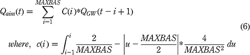
The HBV model version used in this study is HBV light (Seibert, 2005). The model runs on daily time step to simulate daily discharge using daily precipitation, temperature and potential evaporation as inputs. Precipitation is simulated to be either snow if the temperature is below the threshold temperature TT (°C) or rain otherwise. Snow melt is calculated with the degree‐day method (equation (1)). Liquid water within the snow pack refreezes when air temperature fall below TT according to a refreezing coefficient, CFR (−) (equation (2)): Equation 1 Equation 2 Rainfall and snow melt are divided into water filling the soil box and groundwater recharge depending on the relation between water content of the soil box (SM (mm)) and its largest value (FC (mm)) (equation (3)). Actual evapotranspiration from the soil box equals the potential evapotranspiration if SM/FC is above LP (−), while a linear reduction is used when SM/FC is below LP (equation (4)): Equation 3 Equation 4 Groundwater recharge is added to the upper groundwater box (SUZ (mm)). Runoff from the groundwater boxes is computed as the sum of two or three linear outflow equations (K0, K1 and K2 (d−1)) depending on whether SUZ is above a threshold value, UZL (mm), or not (equation (5)). This runoff is finally transformed to give the simulated runoff (mm d−1) (equation (6)). The model has in total ten parameters to be calibrated: Equation 5 Equation 6
WASMOD model
The WASMOD is a conceptual lumped modeling system developed by Xu (2002), and different versions of the model have been widely applied for runoff simulation at catchment, regional and global scales (Gong et al., 2009; Jin et al., 2010; Widen‐Nilsson et al., 2007, 2009; Li et al., 2011, 2012). In this study a monthly time step WASMOD is used which requires monthly values of areal precipitation, potential evapotranspiration and air temperature as inputs. Temperature‐index function is used to separate rainfall rt and snowfall st and then snowfall is added to the snowpack spt (the first storage) at the end of the month, of which a fraction mt melts and contributes to the soil‐moisture storage smt. The soil storage contributes to evapotranspiration et, to a fast component of flow ft and to base flow bt. All the above mentioned processes are governed by six parameters (a1‐a6) and the principal equations for the parameters are presented in Table II.
Model calibration and validation
The parameters of WASMOD and HBV models were determined through the calibration procedure. For HBV model, Monte Carlo procedure was used to investigate the best parameter values using the results of a large number of model runs with randomly generated parameter sets. Using the best parameter set, the first one year period used as a warm up period to initialize the model before actual calibration and the remaining periods were divided in such a way that two‐third of the data was used for the calibration and one‐third of the data was used for validation. In the case of WASMOD, an automatical optimization is used. After the specification procedure, two‐third of the data was used for calibration and the remaining one‐third of the data for validation.
Among the many model performance indicators, the Nash‐Sutcliffe model efficiency coefficient (E) has been widely used to quantitatively describe the accuracy of model output. The coefficient can range from minus infinity to one with higher value indicating better performance and it is defined as: Equation 7 where Qobs and Qsim represent observed and simulated discharge, respectively, and Qobs is observed mean value. The value of E represents the extent to which the simulated value is the better predictor of the observed mean. In addition to Nash‐Sutcliffe model efficiency coefficient (E), root mean square error (RMSE) and relative volume error (RVE) were also applied.
The root mean square error (RMSE) is the measure of differences between values predicted by a model and values actually observed. The root mean square error (RMSE) is defined as: Equation 8 where Qobs and Qsim represent observed and simulated discharge, respectively, and n is a number of observations. Since the errors are squared before they are averaged, it gives relatively high weight to large errors. The value of RMSE can ranges from 0 to ∞ and lower values are better.
Relative volume of error (RVE) tells whether the model simulation is biased as compared with observation. It is defined as: Equation 9 where, Qobs and Qsim represent observed and simulated discharge, respectively.
Result and discussion
Evaluation of model performance in reproducing historical records
Statistical analysis was conducted to evaluate the performance of the models. The result of statistical analysis for the calibration and validation period is presented in Table III. The value of Nash‐Sutcliffe coefficient (E) indicates that both models are performed quite well in all catchments and it ranges from 0.88 to 0.96 for calibration period and from 0.80 to 0.95 for validation period. The corresponding low error (RMSE and RVE) increased the confidence of the models performance to simulate the historical records at acceptable accuracy.
Also, the statistical result shows that no significant difference exists between the two models in reproducing the historical records.
Comparisons of mean monthly runoff values simulated by WASMOD and HBV models with the observed values are shown in Figure 2. There is a good agreement in the mean monthly observed runoff with both model simulations. Our results demonstrate that both models were able to reproduce the dynamics of monthly runoff hydrograph for all catchments.
Generally, the statistical results and visual observation of observed and calculated runoff graph show that both WASMOD and HBV models can reproduce historical monthly runoff series at all tested climate zone catchments with an acceptable accuracy. No significant difference exists between the two models in reproducing the historical records. The main purpose of comparing the observed runoff with model simulated value is to check the capability of the models in reproducing the historical records at acceptable accuracy on different climate zones in order to make sure that the simulations under climate change conditions will be predicted well.
Model simulation corresponding to future climate change scenarios
After calibrating the hydrological models with the historical record, the next step in the investigation was to simulate flows corresponding to future climate conditions. The results were plotted as a percentage of change from the simulated long‐term annual and monthly water balance components, namely runoff, evapotranspiration and soil moisture content. This will help in identifying any specific trend in the change of monthly and annual runoff, actual evapotranspiration and soil moisture storage in the Didessa, Dongjiang and Elverum river basins corresponding to the different future climate change scenarios.
Change in mean annual runoff
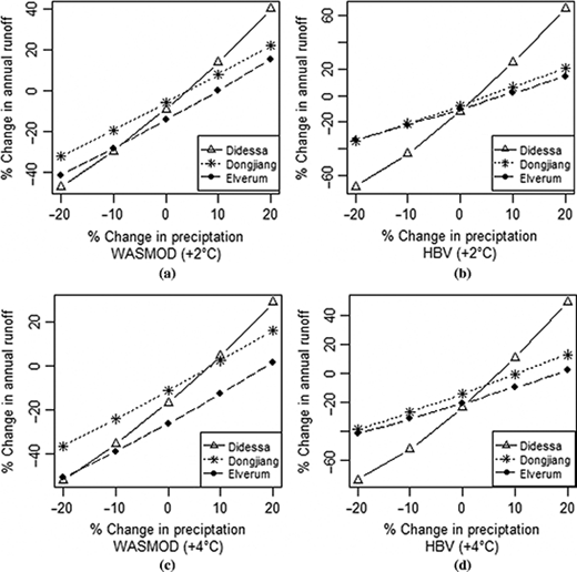
The sensitivity of river basins to the changing precipitation and temperature input is evaluated based on the runoff at the catchment outlet. The scale of the catchment also influences the runoff at the outlet. In order to investigate the impact of precipitation and temperature change on mean annual runoff change at different catchment scales, nested small catchment within the river basins was identified, namely, Shuntian catchment within Dongjiang basin, Dembi catchment within Didessa basin, and Hummelvoll within Elverum basin. Figure 3 shows that the mean annual runoff change using all ten scenarios at different catchment scale. It is seen from the figure that:
The general pattern of annual changes of runoff simulated by both models are somehow similar. Scenarios with decreased precipitation (i.e. scenarios 1, 2, 6, 7) result in decreased runoff for both models and for all catchments regardless of the magnitude of temperature increase (i.e. 2 or 4°C). Scenarios with increased precipitation (i.e. scenarios 4, 5, 9, 10) result in increased runoff for both models and for all catchments except one case. For scenarios 3 and 8 (i.e. precipitation does not change while temperature increases 2 and 4°C, respectively) HBV model shows a decrease in runoff for all the catchment while WASMOD shows a slight increase in runoff for Hummelvoll catchment, which is in a cold region covered with snow for more than a half year.
The magnitude of the runoff change depends on the scenario, the model and the climate region.
More detailed changes of runoff with respect to different scenarios can be seen from Figure 4, which shows that:
Annual runoff change is more sensitive for change in precipitation in Didessa basin (located in the South‐Western of Ethiopia) as compared with other basins under both model predictions (Figure 4). The change ranges from about −65 to +40 percent as simulated by HBV and from about −50 to +30 percent as simulated by WASMOD for the scenarios with temperature increases by 4°C.
On the other hand, the annual runoff change in Dongjiang basin (located in Southeast China) is least sensitive for precipitation change on the annual base.
The change ranges from about −40 to 0 percent as simulated by HBV and from about −40 to +15 percent as simulated by WASMOD. Form Elverum basin the result of HBV is similar with Dongjiang basin and the result of WASMOD shows a slight difference with Dongjiang basin on the annual changes.
Change in mean monthly runoff
Figure 5 shows that:
Large difference exists between two models especially for the scenarios with precipitation decrease.
Dongjiang has smallest seasonal variability whereas Elverum has the largest seasonal variability.
The largest change is observed at Elverum in April, this reflecting the fact that the temperature increase is sufficient enough to cause snow melt so as to create peak runoff.
Change in mean annual evapotranspiration
Similar to the change in annual runoff, the changes in annual evapotranspiration also vary between the regions when climate change scenarios are used to drive the two models. It is seen from Figure 6 that:
There is large difference between models.
The annual actual evapotranspiration change in Elverum basin is highly sensitive for temperature change scenario, whereas for precipitation change scenario, the change is relatively less. This reflects that the limiting factor for evaporation in the area is energy than moisture.
Actual evapotranspiration change in Didessa and Dongjiang basin is more sensitive for precipitation change scenarios than temperature change scenarios on the annual base.
This is due to the fact that moisture is the limiting factor in the regions.
Change in mean monthly evapotranspiration
Figure 7 shows changes in mean monthly actual evapotranspiration (AET). The result indicates that:
There is a remarkable difference between the two models' predictions, scenarios and the regions.
Dongjiang basin has relatively less seasonal variation than the other regions.
Elverum has highest seasonal variations of actual evapotranspiration relative to the other regions. The basin is more sensitive for temperature change scenario than precipitation change scenario.
Didessa basin has highest seasonal variation for precipitation increase scenarios, while seasonal variation is less for precipitation decrease scenarios.
Change in mean annual soil moisture storage
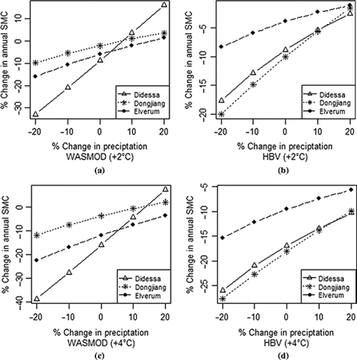
The percent change of mean annual soil moisture in response to precipitation and temperature change scenarios are shown in Figure 8. In general, Figure 8 shows that:
There is large difference between the two models.
The difference in annual soil moisture change simulated by WASMOD model is larger than HBV simulation in Didessa basin as compare to the other basins.
Annual soil moisture change is less sensitive for precipitation change scenario in Elverum basin under both model predictions, while Dongjiang basin also less sensitive for precipitation change scenario under WASMOD simulation but relatively the sensitivity increases under HBV model simulation.
The magnitude changes in mean annual soil moisture content of the three basins are similar when the change in precipitation increases by 20 percent.
But when precipitation reduced by 20 percent, the mean annual soil moisture content reduced by far in the case of Didessa and Dongjiang basins as compared with Elverum basin.
Change in mean monthly soil moisture storage
Mean monthly soil moisture content change detected by the two models for the selected climate change scenarios were plotted in Figure 9. The figure shows that:
The patterns of change as well as the magnitudes of change between the two models are quite different.
Dongjiang has the smallest seasonal soil moisture variation whereas Didessa has the largest seasonal variation for different precipitation and temperature change scenarios.
In Didessa basin, soil moisture content is more sensitive for precipitation change scenarios as compare to temperature change scenarios.
Implication of the study on climate change management
This section highlights key findings and policy implications that would be useful for policy makers to consider with respect to climate change adaptation. The knowledge of changes of hydrological variables due to climate change will be important to develop resilience infrastructure and proper resource management in a given region. For reliable projection of potential ranges of impacts from scenarios of future change, technical improvement of hydrological models is a valuable strategy.
The hydrological impact of climate change will vary in different regions. In this particular study, the vulnerability of different representative basins investigated through hydrological modeling by using the same climate change scenario.
As retrieved from the study, in tropical climatic region (Didessa basin), the seasonal as well as annual runoff variation is very high for increasing climate change scenarios. If we focus on precipitation decrease and temperature increase scenarios as most global circulation models predicted for the region, the region will affected by moisture stress. This projected future water stress and scarcity will have serious impacts on the socio‐economic development of the countries affected and will likely adversely affect their food production levels and development plans. Understanding the magnitude of situation through hydrological modeling will help to create appropriate adaptation strategies.
In the polar region (Elverum basin), the variation of annual runoff is less whereas seasonal variability is very high. As temperatures rise due to climate change in the region, winter snow melts increases which lead to a change in the timing of the peaks runoff. Understanding the magnitude of seasonal variability and the time of peak flow in the region through hydrological modeling, will help for hydropower dams operational plan, flood control strategic plan. On the other hand, reduction of low flows in summer and autumn may have large impacts on water resource availability. Therefore, hydrological modeling of climate change will help as a tool for climate change adaptation strategies.
Conclusion
The main focus of the study is to test the magnitude differences one can expect when using different hydrological models to simulate hydrological response of climate changes in different climate zones as compared to their capacities in simulating historical water balance components. To achieve the main goal two well‐known models (i.e. HBV and WASMOD) are applied on six catchments with different size and climate regions, i.e. two in Norway with seasonal snow coverage, two in subtropical region in Southeast China and two in Southwest Ethiopia with least intra‐annual temperature variations. The following conclusions are drawn from the study:
The result of statistical analysis for calibration and validation shows that both models can reproduce the historical runoff with acceptable accuracy for each basin.
Large differences exist between the two models under climate change conditions when climate change scenarios incorporated to predicted runoff, actual evapotranspiration and soil moisture especially at the monthly time scales.
The differences depend on the models, climate change scenarios, the seasons, and the regions where the study is conducted and the hydrological variables under examination. In general, the basins in Southwest Ethiopia show a largest change in annual runoff and annual soil moisture. While the catchments in Norway show largest increase in annual evapotranspiration with the increase of temperature, indicating that this region is more of energy limited region for evapotranspiration. At monthly time scale, large differences are found for the changes in runoff, evapotranspiration and soil moisture between the results of the two models and between the study regions. In general monthly changes in runoff and evapotranspiration in the seasonally snow covered basins in Norway have shown largest seasonal pattern, while the monthly changes in the basins in subtropical region in Southeast China have shown least seasonal pattern.
Remarkable differences between the two models results are found for all the catchments when climate change scenarios are used to drive the models, and the largest differences are found at monthly time scale.
The results of this study demonstrate that, hydrological impact of climate change predicted by any particular hydrological model represents only the result of that model for the specific region where the study is conducted. The purpose of this paper was to demonstrate how two equally well calibrated models gave different hydrological response to hypothetical climatic scenarios. It is important to emphasize that the climatic scenarios used as input for the simulations, represents significant extrapolation of temperature and precipitation used for parameter calibration of the hydrological models applied in this study. The diverging responses indicate clearly the limitation in lumped hydrological modeling. Extrapolation of driving forces (temperature and precipitation) beyond the range of parameter calibration yields unreliable response. It is beyond the scope of this study to reduce this model ambiguity, but reduction of uncertainty is a challenge for further research.
Acknowledgements
The work presented in this paper was supported by the Department of Geosciences, University of Oslo, through the Norwegian Research Council (RCN) Environment and Development Programme (FRIMUF) project number 171783. The authors are grateful to the Ministry of Water Resource and National Meteorology Agency of Ethiopia, and Norwegian Water Resource and Energy Directorate (NVE), for their collaboration in providing meteorological and stream flow data. The authors gratefully acknowledge Professor Yongqin David Chen, the Chinese University of Hong Kong, who provided hydrological data for the Dongjiang basin through the Project no. CUHK4627/05H of the Research Grants Council of the Hong Kong Special Administrative Region, China.








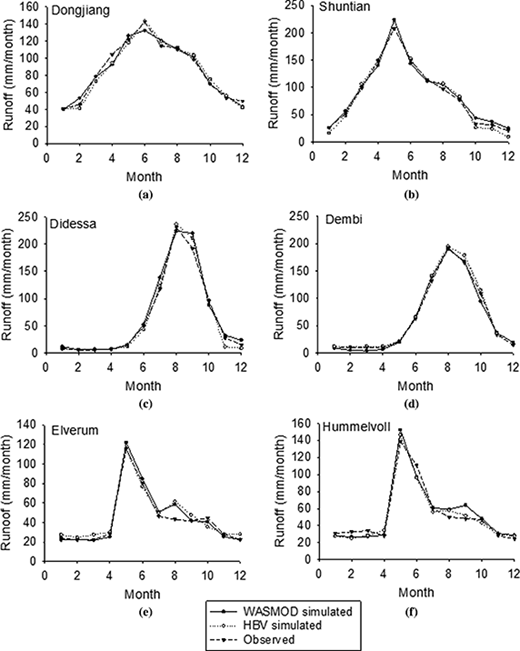
Comparisons of mean monthly observed runoff with WASMOD and HBV simulated runoff in each catchment
Comparisons of mean monthly observed runoff with WASMOD and HBV simulated runoff in each catchment
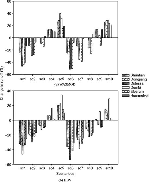
Mean annual runoff change estimated by WASMOD model (upper graph) and HBV model (lower graph) using ten scenarios in different catchments
Mean annual runoff change estimated by WASMOD model (upper graph) and HBV model (lower graph) using ten scenarios in different catchments
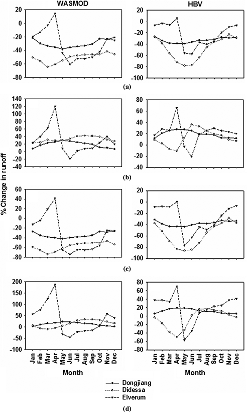
Comparison of mean monthly change in runoff simulated by WASMOD (left graph) and HBV (right graph) for scenario 1 – a, scenario 5 – b, scenario 6 – c, scenario 10 – d
Comparison of mean monthly change in runoff simulated by WASMOD (left graph) and HBV (right graph) for scenario 1 – a, scenario 5 – b, scenario 6 – c, scenario 10 – d
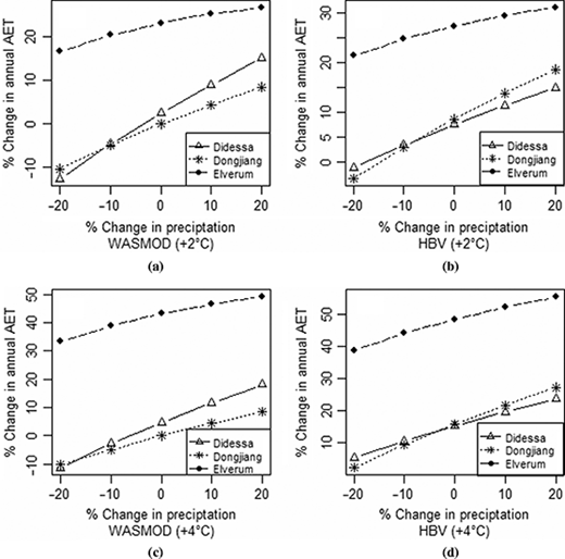
Mean annual actual evapotranspiration change simulated by WASMOD and HBV models
Mean annual actual evapotranspiration change simulated by WASMOD and HBV models
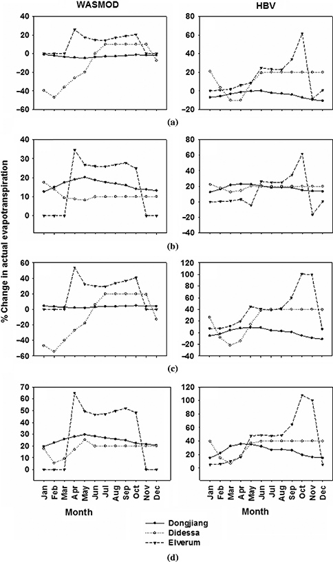
Comparison of mean monthly change in actual evapotranspiration simulated by WASMOD (left graph) and HBV (right graph) for scenario 1 – a, scenario 5 – b, scenario 6 – c, scenario 10 – d
Comparison of mean monthly change in actual evapotranspiration simulated by WASMOD (left graph) and HBV (right graph) for scenario 1 – a, scenario 5 – b, scenario 6 – c, scenario 10 – d
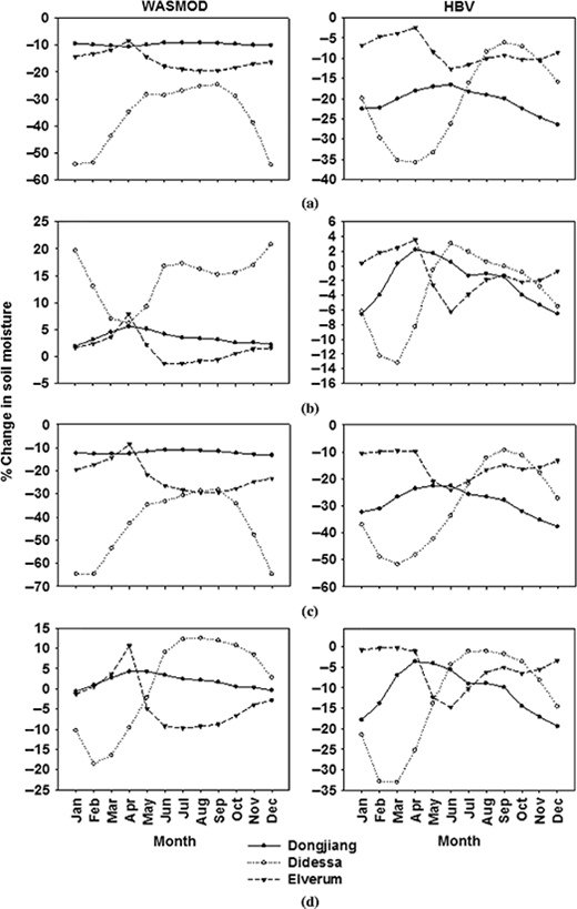
Comparison of mean monthly change in soil moisture simulated by WASMOD (left graph) and HBV (right graph) for scenario 1 – a, scenario 5 – b, scenario 6 – c, scenario 10 – d
Comparison of mean monthly change in soil moisture simulated by WASMOD (left graph) and HBV (right graph) for scenario 1 – a, scenario 5 – b, scenario 6 – c, scenario 10 – d

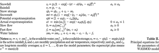
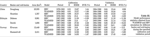
Model performance statistics obtained from WASMOD and HBV simulation for different basins and sub‐basins during the specified calibration and validation period
Model performance statistics obtained from WASMOD and HBV simulation for different basins and sub‐basins during the specified calibration and validation period
References
About the authors
Fasil Ejigu Eregno is a student at the Department of Plant and Environmental Sciences, Norwegian University of Life Sciences. His main areas of interest are hydrological modeling at regional and catchment scale; water quality modeling; and erosion and sediment transport. Fasil Ejigu Eregno is the corresponding author and can be contacted at: efasilejigu@yahoo.com
Chong‐Yu Xu is a Professor of Hydrology at the Department of Geosciences, University of Oslo. His main areas of interest are related to hydrological modelling at global, regional and catchment scales; modelling of hydrological impact of climate and environment changes at global, regional and catchment scales; regional evapotranspiration and its role in linking climatic and hydrological system; regionalization of hydrological variables and model parameters; uncertainty analysis; and time series analysis.
Nils‐Otto Kitterød is Associate Professor in Hydrology at the Department of Plant and Environmental Sciences, Norwegian University of Life Sciences. His main areas of interest are related to soil water, groundwater, transport of contaminants, geostatistics, and stochastic simulation.

