


– This study aims to investigate the effects of climate change on harvestability for sugarcane-growing regions situated between mountain ranges and the narrow east Australian coastline.
– Daily rainfall simulations from 11 general circulation models (GCMs) were downscaled for seven Australian sugarcane regions (1961:2000). Unharvestable days were calculated from these 11 GCMs and compared to interpolated observed data. The historical downscaled GCM simulations were then compared to simulations under low (B1) and high (A2) emissions scenarios for the period of 2046-2065. The 25th, 50th and 75th percentiles of paired model differences were assessed using 95 per cent bootstrapped confidence intervals.
– A decrease in the number of unharvestable days for the Burdekin (winter/spring) and Bundaberg (winter) regions and an increase for the Herbert region (spring) were plausible under the A2 scenario. Spatial plots identified variability within regions. Northern and southern regions were more variable than central regions.
– Changes to the frequency of unharvestable days may require a range of management adaptations such as modifying the harvest period and upgrading harvesting technologies.
– The application of a targeted industry rainfall parameter (unharvestable days) obtained from downscaled climate models provided a novel approach to investigate the impacts of climate change. This research forms a baseline for industry discussion and adaptation planning towards an environmentally and economically sustainable future. The methodology outlined can easily be extended to other primary industries impacted by wet weather.
1. Introduction
1.1 Climate impacts on the Australian sugar industry
Prior knowledge of climate conditions for the upcoming harvest season would influence the decision-making process in the Australian sugar industry. The sugarcane harvest season in Australia starts in the drier Austral winter months usually around June and extends through to the end of spring, with the aim to finish before the start of the summer wet season (December-February) (Figure 1). If excessive delays occur during harvest, the harvest window will be pushed further into the monsoon season. Such delays can cause crop stand over and major losses to farmer profits. Everingham et al. (2011) demonstrated that annual profits up to AUD1.9 million could be delivered through application of seasonal climate forecasting, to identify optimal harvest start dates for the Herbert sugarcane region. In the same region, Antony et al. (2002) identified that the 1998/1999 La Niña cost the industry AUD19 million. It is vital that industry decision-makers have knowledge about likely rainfall-related impacts during the harvest season.
The sugar industry is mindful of seasonal rainfall projections; however, a large number of small rainfall events can be more detrimental than a single large event (Everingham and Reason, 2011). An important method for assessing climatic impacts on sugarcane harvesting is to consider the frequency of rainfall events. Everingham and Reason (2011) investigated “wet spell” frequency during the autumn and winter harvest period in New South Wales (NSW). The study identified that five-day “pentads” with above median rainfall were significantly correlated with high seasonal rainfall.
A “wet days” rule for classifying rainfall events which would stop harvest in Queensland sugarcane-growing regions has been identified (Muchow et al., 1996) and integrated with probabilistic seasonal forecasting (Everingham et al., 2002, 2011). It was concluded that seasonal climate forecasting could add value to decisions influenced by high rainfall events late in the harvest season (October-November). Everingham et al. (2011) used the harvest disruption rule in developing a forecast-driven management plan that resulted in an increase in revenue in the order of AUD500,000. The lessons learnt from such climate variability studies can be applied to improve climate change projections that focus largely on seasonal or monthly mean projections.
The “2007 Climate Change in Australia” technical report documented rainfall projections from 25 climate models (Pearce et al., 2007). The median or “best estimate” of rainfall projections decreased by approximately 2 to 20 per cent for most of coastal Queensland and NSW during the harvest season for the year 2050. The 2007 technical report also concluded that an increase in daily precipitation intensity across Australia was likely but did not directly consider the frequency of these events.
Globally, climate change studies have suggested an increase in the occurrences of extreme rainfall events (Kharin et al., 2007). Similar results have been found for Australia (Alexander and Arblaster, 2009). Heavy rainfall events can cause nutrient runoff, soil erosion and flooding events (Park, 2003), as well as disrupting harvest. Despite this, impact analyses for sugarcane in Australia have predominantly focussed on implications for cane yield. Impact studies have projected both increases in yield (Webster et al., 2009; Park et al., 2007; Biggs et al., 2012) and decreases depending on the scenario and management practices used (Park et al., 2007; Biggs et al., 2012).
1.2 General circulation models and downscaled climate data
Climate change has triggered a global push for enhanced climate datasets and realistic models that describe climate variables such as rainfall and temperature. Phase 3 of the World Climate Research Programme’s (WCRP) Working Group on Coupled Modelling (WGCM), Coupled Model Intercomparison Project (CMIP3), collected a range of general circulation models (GCMs). This dataset is known as the “WCRP CMIP3 multi-model dataset” (www-pcmdi.llnl.gov/ipcc/about_ipcc.php). The data were collected by the Program for Climate Model Diagnosis and Intercomparison (PCMDI) and represent a range of climate change experiments based on different climate scenarios (Meehl et al., 2007).
Rainfall variability is particularly affected by small-scale climate cycles and local topography (Timbal and Arblaster, 2006; Garnaut, 2008). The abrupt change in geography (Figure 2) and sub-tropical nature of sugarcane-growing regions in Australia produce a climatology that is subject to high spatial and temporal variability (Lough, 1991; Tularam and Ilahee, 2010) that may not be properly reflected in GCMs. Downscaling GCM data offers a solution to this problem by providing climate data at a high spatial resolution.
Downscaling processes relate local climatic variables to large-scale atmospheric data (Hewitson and Crane, 1996) and have found diverse application in regional impact studies around the world, such as climate extremes in southern China (Yang et al., 2012), landslides in Thailand (Chiang and Chang, 2011) and water quality in India (Rehana and Mujumdar, 2012). Rainfall studies in Australia have used dynamical downscaling methods such as the Conformal-Cubic Atmospheric Model (Bennett et al., 2012) and statistical methods such as the analogues methodology (Timbal et al., 2011) and non-homogeneous hidden Markov model (Fu et al., 2013). The appropriate choice of downscaling method often depends on the type of analysis being performed. Many comparisons between methods are available in the literature. Frost et al. (2011) compare downscaling previously used in Australia, while Fowler et al. (2007) offer a review of downscaling techniques used in hydrological impact studies, including comparisons between statistical and dynamical downscaling.
1.3 Paper objectives
Use of the wet days rule and high spatial resolution climate projections will produce informative climate change impact analysis for industry decision-makers. Therefore, the objectives of this paper are to use downscaled climate data to:
assess the ability of individual GCMs to model unharvestable days in the Australian sugarcane industry;
investigate the multi-model mean change simulated spatially; and
investigate the implications of climate change on harvestability, as described by the 25th, 50th and 75th percentiles of changes in the number of unharvestable days, as simulated by 11 GCMs.
2. Data generation
2.1 Interpolated rainfall
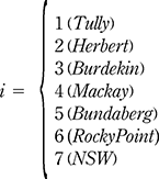
Daily rainfall data were obtained for seven sugar sugarcane-growing regions across eastern Australia (Figure 2). Individual pixels of 0.05 × 0.05 decimal degrees were identified as growing sugarcane for each region (Tully: 77 pixels, Herbert: 58 pixels, Burdekin: 64 pixels, Mackay: 133 pixels, Bundaberg: 107 pixels, Rocky point: 7 pixels and NSW: 76 pixels). Sugarcane-growing regions were described by land-use maps from the Department of Environment and Research Management and local industry spatial data. Data from the Australian Water Availability Project (AWAP) were used as baseline historical data for the period of 1961-2000. The AWAP data represent spatially interpolated weather station data, also on a 0.05 × 0.05 decimal degree grid (Jones et al., 2009).
2.2 Historical GCM simulated data
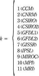
GCM outputs for the period of 1961-2000 were downscaled under the 20C3M scenario, which used observed trends in greenhouse gas emissions for the twentieth century (PCMDI, 2002). The CMIP3 database (available at: www-pcmdi.llnl.gov./ipcc/info_for_anaysts.php#getting_started) houses data from 25 GCMs. Eleven GCMs that had rainfall on a daily time step were selected from the CMIP3 database. These GCMs are identified as Canadian Climate Centre, Centre National de Recherches Météorologiques (CNRM) (Metro-France), CSIRO (Commonwealth Scientific and Industrial Research Organisation), CSIRO2, GFDL1 (Geophysical Fluid Dynamics Lab), GFDL2, The Goddard Institute for Space Studies GISS-ER GCM (GISSR) (NASA/Goddard Institute for Space Studies), Institute Pierre Simon Laplace, MIROC (Centre for Climate Research), MPI (Max Planck Institute for meteorology), The German Climate Computation Centre (DKRZ), MRI (Meteorological Research Institute).
2.3 GCM future projections
Rainfall projections for the 11 GCMs were extracted for the period of 2046-2065. Two projected climate scenarios were used – the B1 and A2 scenarios, as described by the International Panel on Climate Change (IPCC). The B1 scenario focussed on a future with “[…] emphasis on global solutions to economic, social and environmental sustainability […]” (Nakicenovic and Swart, 2000) and was used to represent a low emissions future. The A2 scenario outlines a future of high economic and population growth and was used to represent a high emissions future.
2.4 Analogue downscaling applied to GCM data
GCM data were downscaled using the Australian Bureau of Meteorology (BoM) analogues methodology (Timbal et al., 2009). The availability of high-resolution GCM data across Australia (Timbal et al., 2011) made the analogues method ideal for regional climate change impact studies. Furthermore, the cane industry in Australia has previously made use of probability forecasts based on matching phases of the southern oscillation index and El Niño-La Niña southern oscillation (Everingham et al., 2002, 2011). Therefore, the industry had a familiarity with matching similar climates (analogues) for probability analysis. This methodology has been used in impact analyses in Australia, where high-resolution rainfall data were required (Liu et al., 2011).
High-quality reanalysis data from the National Centers for Environmental Protection and National Center for Atmospheric Research Reanalysis datasets (NNR) (Kalnay et al., 1996) were used in conjunction with AWAP data to generate a downscaling model. Analogues were chosen using a Euclidean closest neighbour approach. The downscaling model was built based on large-scale predictors that best described daily rainfall. Optimisation accounted for domain size (geographic area considered), calendar window (number of days before and after model date) and anomalies (Timbal et al., 2009). Finally, the downscaling model was applied to GCM outputs by matching analogues from individual GCMs to the NNR data for sugarcane-growing regions along the east Australian coast.
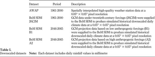
The sugarcane-growing areas analysed herein, fell within the Queensland and Mid-East coast climate regions, as described by Timbal et al. (2011). Large-scale rainfall was the only successful predictor of localised rainfall in the Queensland climate region. The Mid-East region used an optimum combination of predictors including, but not limited to, relative humidity at 850 hPa, mean sea level pressure and the meridional wind at 850 hPa. The Mackay sugarcane-growing region (Region 4) was found to lie on the border between the Queensland and Mid-East coast climate regions. For continuity, all of Mackay was treated as being part of the Queensland climate region. Table I lists the downscaled rainfall datasets used in the generation of harvestability data.
2.5 Defining unharvestable days
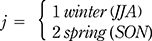
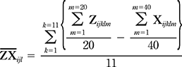
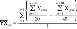
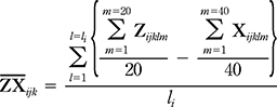
The definition of an unharvestable day (Muchow et al., 1996) applied the following rule: If > 10 to ≤ 20 mm of rain occurred in one day, then that day was assumed to be unharvestable. If > 20 to ≤ 40 mm of rain occurred, then that day and the next were assumed to be unharvestable. If > 40 mm of rain occurred, then that day and the next two days were assumed to be unharvestable. This rule was applied to the four downscaled rainfall datasets (Table I). The total number of unharvestable days was calculated for the downscaled AWAP (a i j l m), BoM Statistical Downscaling Model (SDM) 20C3M (x i j k l m), BoM SDM B1 (y i j k l m) and BoM SDM A2 (z i j k l m) datasets. Calculations were performed for each region: Equation 1
for each season: Equation 2
and for GCM: Equation 3
pixel l = {1, 2 […], }, where l i is the number of pixels in region i, and year m = {1, 2 […], m 0}, where m 0 is the total number of years analysed.
3. Analysis method
The Kolmogorov Smirnov (KS) test was used to assess the ability of downscaled GCM simulations of unharvestable days to reproduce the AWAP distribution of unharvestable days. Spatial plots were produced of the multi-model temporal mean of paired differences in the number of unharvestable days. Regional spatio-temporal means were also produced, and the distribution of paired model differences was assessed using confidence intervals. Figure 3 outlines the methodological process.
3.1 Analysis of empirical cumulative distribution functions
Empirical cumulative distribution functions were produced from the spatial mean number of unharvestable days for AWAP: Equation 4
and BoM SDM 20C3M data. The KS test function in the R statistical software programme (R Development Core Team, 2011) was used to compare distribution functions of AWAP {a¯ i j1, a¯ i j2, …, a¯ i j40} and BoM SDM 20C3M {x¯ i j k1, x¯ i j k2, …, x¯ i j k40} for each region, season and GCM combination. A p value of 0.05 was used as a cut-off for significantly different distributions.
3.2 Analysis of multi-model means and the distribution of downscaled GCMs
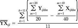
The multi-model mean of paired differences were calculated between the 40-year period of 1960-2000 and 20-year period of 2046-2065, for both low (BoM SDM B1): Equation 5
and high (BOM SDM A2): Equation 6
emission scenarios. These multi-model means were plotted for each region and season combination to visualise spatial variability in unharvestable days. For example, in Region 1, which had 77 pixels, the points Inline Equation 1 were displayed.
Regional spatio-temporal differences were then calculated as the spatial mean of paired differences in temporal means for the low: Equation 7
and high: Equation 8
emissions scenarios.
Bootstrapped confidence intervals (95 per cent) were produced for the 25th, 50th and 75th percentiles of the paired differences in spatio-temporal means (Good, 1997). Consider, for example, the 25th percentile of spatio-temporal mean paired differences, under the high emissions scenario for region (i) and season (j):
The paired differences of the downscaled GCMs were randomly selected with replacement to form a new set of 11, e.g. (Inline Equation 2, Inline Equation 3, Inline Equation 4, Inline Equation 5, Inline Equation 6, Inline Equation 7, Inline Equation 8, Inline Equation 9, Inline Equation 10, Inline Equation 11, Inline Equation 12).
The 25th percentile was calculated for this random selection, and the process was repeated another 999 times.
Confidence intervals were calculated as the middle 95 per cent of the ordered 1,000 sample percentiles.
The process was repeated for the 50th and 75th percentiles, for each region and season combination. Both the multi-model mean and percentile analysis assume the GCMs are independent. This assumption was considered valid, as the 11 GCMs analysed formed a reasonable spread across the “families” of GCMs based on rainfall, identified by Masson and Knutti (2011).
4. Results
4.1 Analysis of empirical cumulative distribution functions
For all regions and seasons, only the MIROC and CSIRO2 downscaled GCMs produced distribution functions that were not significantly different from that of the AWAP unharvestable days (p value > 0.05 for both MIROC and CSIRO2). In Region 1, downscaled MPI and CSIRO GCMs produced KS p values of < 0.05 in winter. However, in spring, there was insufficient evidence to suggest a difference between AWAP and MPI/CSIRO distribution functions (Figure 4(a)). Distribution functions of downscaled GCMs for Region 7 (Figure 4(b)), more closely represented AWAP data in winter, when compared to Region 1.
4.2 Spatial analysis of multi-model means
The multi-model mean of all GCMs simulated a decrease in winter and an increase in spring in most regions (Figure 5). Simulated changes were generally similar under the A2 and B1 scenarios. Regions in the far north and south simulated increases more often than central regions such as the Burdekin and Mackay. Spatial variations were also evident within regions. For example, Region 1 (Figure 6) was one of the most spatially varied regions, whereas Region 3 simulated no spatial variation. Region 2 was not as spatially variable as Region 1, but projections were made for both an increase (northern districts) and decrease (southern district) in spring (data not shown).
4.3 Distribution of spatio-temporal mean differences
Few regions simulated notable changes when the 25th, 50th and 75th percentiles were analysed (Figure 7). For both the low (B1) and high (A2) scenarios, 95 per cent confidence intervals of the spring 75th percentile captured positive values in Regions 1, 2, 5, 6 and 7. The 25th percentile in winter captured negative values for Regions 5, 6 and 7. However, there were only three cases in which confidence intervals of the 50th percentile did not capture a zero value. These cases all occurred under the A2 scenario:
In Region 2, the 95 per cent confidence interval of the 50th percentile captured only positive values for spring.
In Region 3, the 95 per cent confidence interval of the 50th percentile captured only negative values for spring and winter.
In Region 5, the 95 per cent confidence interval of the 50th percentile captured only negative values for winter.
5. Discussion
A spread in cumulative distribution functions produced from the downscaled GCMs relative to AWAP historical simulations was observed. This divergence between GCMs supported the need to analyse the distribution of simulations rather than any single model. Although both MIROC and CSIRO2 replicated historical data well, these two GCMs did not always agree on the projected direction of change. For example, under both B1 and A2 scenarios, the MIROC GCM projected an increase in unharvestable days for spring in Tully (Region 1), whereas the CSIRO2 GCM projected a decrease (data not shown). Given the uncertainty that surrounds GCM projections, we considered outputs from an ensemble of GCMs.
The lower (B1) and higher (A2) emission scenarios both exhibited spatial variability in changes to the frequency of unharvestable days within regions. For regions in the far north and south, the multi-model mean reflected a higher spatial variability than more central regions. For example, the Herbert region (Region 2) projected an increase in northern districts and a decrease in southern districts of the region. It may be necessary to implement a geographically based harvest schedule in regions like the Herbert. More “at risk” districts (where the number of unharvestable days is projected to increase), such as in the north of the Herbert, could be harvested earlier than the southern districts to minimise the impact of increased unharvestable days late in the harvest season. Northern regions may also require greater access to wet weather harvesting equipment if yields increase as projected in recent studies such as Biggs et al.’s (2012) study. Harvesting on “wet” days would help complete the harvest before the start of the summer monsoon season.
Both the B1 and A2 scenarios simulated similar trends based on a 95 per cent confidence interval. Confidence intervals under the higher (A2) scenario are important for industry to consider, as current climate projections suggest a future climate that closely resembles a higher emissions scenario (Sheehan, 2008). Using confidence intervals, Everingham et al. (2013) considered an increase in summer rainfall plausible for the Burdekin under the A2 scenario. Although the number of unharvestable days is projected to decrease, if summer rainfall were to increase, it may still be necessary for industry to consider how to complete the harvest before the monsoon season starts. By rescheduling the harvest period for an earlier start, the projected higher yields could be harvested earlier. This would help mitigate some of the risks of either an increased frequency of unharvestable days or an increase in summer rainfall.
There are many negative impacts associated with high-intensity rainfall events such as nutrient runoff, soil erosion and flooding. Simulated increases in the number of unharvestable days parallel trends towards an increase in extreme weather events reported in global (Kharin et al., 2007) and Australian (Alexander and Arblaster, 2009) studies. Nutrient runoff, soil erosion and flooding events associated with increases in high-intensity rainfall may be partially offset by adopting green cane harvesting and improving drainage (Park, 2003). Nutrient runoff is of particular importance in northern regions because of the potential impact on the nearby Great Barrier Reef. This has led to investigations of how to manage fertilizer applications under a changing climate (Skocaj et al., 2013).
6. Conclusion
The sugarcane-growing regions of eastern Australia are geographically heterogeneous and are subject to spatially and seasonally variable rainfall. High-resolution climate change simulations allow spatial differences to be identified within and between harvest regions. Unharvestable days due to wet weather disrupt the harvest season and can have adverse economic consequences. The impacts of climate change may be mitigated, if the industry decision-making process can be influenced by climate projections. The economic effects of adapting to climate change also need to be considered as part of developing any climate change management strategy.
Downscaled GCMs projected under low (B1) and high (A2) emissions scenarios were compared to simulations under twentieth-century forcings (20C3M). The 25th, 50th and 75th percentiles of differences were assessed using 95 per cent bootstrapped confidence intervals. Spatial variability between and within regions was also investigated. There was little evidence to support changes in the number of unharvestable days for most regions. However, A decrease was considered plausible in the Burdekin (winter and spring, A2) and Bundaberg (winter, A2). An increase in the Herbert region (spring, A2) was also considered plausible. This is important to the industry, as it may result in a shortening of the current harvest window. Downscaled GCMs cannot be considered as definite predictions of the future climate. However, a distribution of model projections can provide valuable information to industry decision-makers by identifying regions and seasons with high model agreement on the direction of change. Future research may take advantage of improved GCMs such as the CMIP5 database.




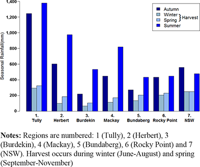
Regionally averaged seasonal rainfall (mm) for the period of 1961-2000 for seven sugarcane-growing regions in Eastern Australia
Regionally averaged seasonal rainfall (mm) for the period of 1961-2000 for seven sugarcane-growing regions in Eastern Australia
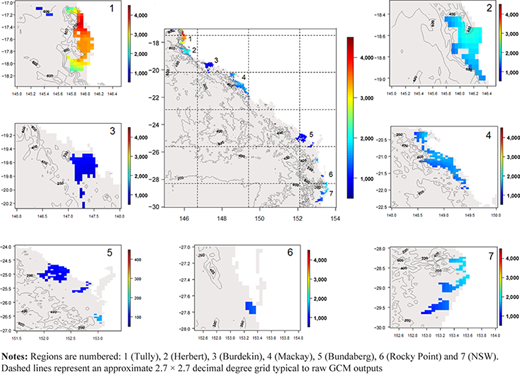
Elevation contours (m) and average total annual rainfall (mm) for the period of 1961-2000 at a 0.05 × 0.05 decimal degree pixel resolution
Elevation contours (m) and average total annual rainfall (mm) for the period of 1961-2000 at a 0.05 × 0.05 decimal degree pixel resolution
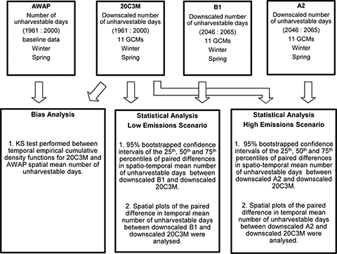
A flowchart of the analysis method
A flowchart of the analysis method
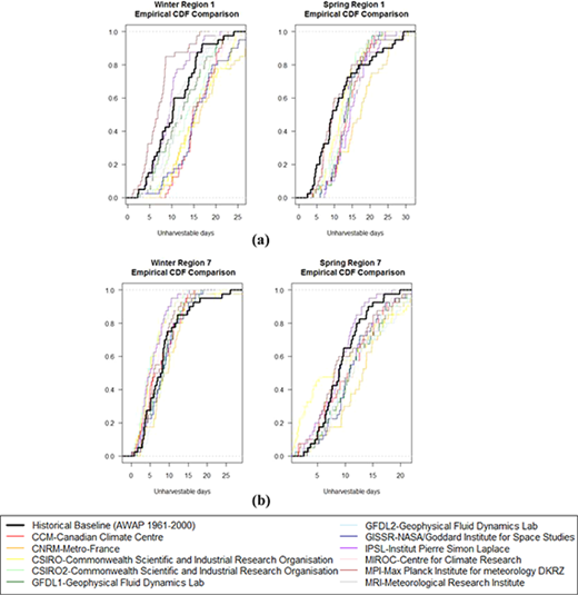
Cumulative distribution functions of unharvestable days for AWAP (black line) and downscaled GCMs (coloured) for the (a) Tully and (b) NSW regions
Cumulative distribution functions of unharvestable days for AWAP (black line) and downscaled GCMs (coloured) for the (a) Tully and (b) NSW regions
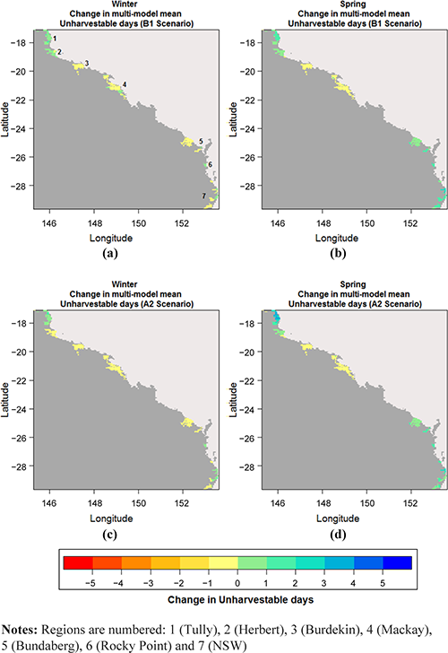
Differences in the multi-model temporal mean number of unharvestable days for high (a), (b) and low (c), (d) emission scenarios in winter (a), (c) and spring (b), (d). Differences compare the periods of 1961-2000 and 2046-2065. Positive values reflect a simulated increase unharvestable days, and negative values reflect a simulated decrease
Differences in the multi-model temporal mean number of unharvestable days for high (a), (b) and low (c), (d) emission scenarios in winter (a), (c) and spring (b), (d). Differences compare the periods of 1961-2000 and 2046-2065. Positive values reflect a simulated increase unharvestable days, and negative values reflect a simulated decrease
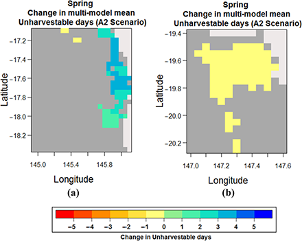
Differences in the multi-model temporal mean number of unharvestable days for high emission scenario in winter for Regions 1 (a) and 3 (b). Differences compare the periods of 1961-2000 and 2046-2065. Positive values reflect a simulated increase in unharvestable days, and negative values reflect a simulated decrease
Differences in the multi-model temporal mean number of unharvestable days for high emission scenario in winter for Regions 1 (a) and 3 (b). Differences compare the periods of 1961-2000 and 2046-2065. Positive values reflect a simulated increase in unharvestable days, and negative values reflect a simulated decrease
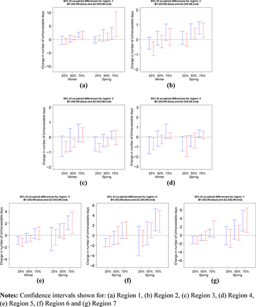
Ninety-five per cent bootstrapped confidence intervals on the 25th 50th and 75th percentiles of the change in unharvestable days. Differences in the spatio-temporal means for 11 GCMs were calculated between the periods of 2046-2065 and 1961-2000 for the B1 (blue) and A2 (red) scenarios
Ninety-five per cent bootstrapped confidence intervals on the 25th 50th and 75th percentiles of the change in unharvestable days. Differences in the spatio-temporal means for 11 GCMs were calculated between the periods of 2046-2065 and 1961-2000 for the B1 (blue) and A2 (red) scenarios
References
About the authors
Justin Sexton currently works as a Research Officer for the School of Engineering and Physical Sciences, James Cook University in Townsville Australia. He completed his bachelor’s degree (Mathematics) at James Cook University in 2010 and has recently (2013) started master’s degree (Mathematics) focussing on statistical calibration of a sugarcane crop model.
Dr Yvette Everingham completed her PhD in 1998 in the field of pattern prediction methods and commenced a four-year term with Australia’s CSIRO as a climate impacts scientist. In 2003, she joined James Cook University as a full-time Lecturer in statistics in the Faculty of Science and Engineering. Today, her research involves solving real-world practical problems with a strong emphasis towards enhancing sustainability practices through the application of quantitative techniques. She currently holds a position as a Senior Lecturer in the School of Engineering and Physical Sciences and is a member of the Centre for Terrestrial Environmental and Sustainability Science, both at James Cook University, Townsville, Australia.
Bertrand Timbal is a Scientist with the Australian Bureau of Meteorology (BoM) based in the Centre for Australian Weather and Climate Research (CWACR) – a joint partnership between the CSIRO and BoM. He has more than 20 years of experience in dealing with climate change simulations and developing methodologies to provide local scale information relevant to impact studies, including the statistical downscaling model used in this application.
The authors would like to thank Yang Wang and Alex Evans for their help with data acquisition. Rodney Neilson, John Markley, Paul Brown, Ben Mayo, Dale Thomas and Jack Katzfey for help with identification of sugarcane-growing regions. The authors acknowledge the international modelling groups for providing their data for analysis, the PCMDI for collecting and archiving the model data, the Joint Scientific Committee (JSC)/Climate and Ocean Variability, Predictability and Change (CLIVAR) WGCM and their CMIP and Climate Simulation Panel for organising the model data analysis activity and the IPCC WG1 TSU for technical support. The IPCC Data Archive at Lawrence Livermore National Laboratory is supported by the Office of Science, USA Department of Energy. This project was funded by the Sugar Research and Development Corporation.

