Dynamics of optimal carbon prices with inter-temporal regulation

Policymakers establish cap-and-trade systems to reduce emissions. The way in which these systems reduce emissions is by establishing a mandatory cap that allows regulated firms to comply with the cap in a flexible manner through the use of emission permits and abatement. This market-based policy instrument provides flexibility, which has led many countries to launch permit-trading schemes. For example, the USA has an Acid Rain Program (ARP) to regulate SO₂ and the NO_x Budget Trading Program in the northeast region; it is well-known that emissions have been reduced substantially over the course of decades through these programs. In addition, the EU Emission Trading Scheme (EU-ETS) is recognized as a representative system to control carbon dioxide emissions, and this carbon-trading system is expected to expand to other countries to protect the planet from climate change. The cap set by the EU-ETS Directive has been administered by an environmental regulatory office. In this paper, we will use this carbon trading scheme as the representative cap-and-trade system for our analysis due to its large market size and its promising future as a worldwide trading market.

In this paper, we use the stochastic and dynamic carbon pricing model to determine the regulation effect of banking and borrowing on prices. Our model incorporates the environmental damage function to derive a socially desirable price level. Price simulation can then help policymakers choose the most appropriate banking and borrowing rule because they know what price level is desirable from the perspective of the social planner.

The regulation of banking and borrowing in the emissions-trading market has received considerable attention in the literature (Rubin, 1996; Kling and Rubin, 1997; Schleich et al., 2006; Cason and Gangadharan, 2006). From the principle of ETS, market participants can alternatively borrow permits from the future in addition to purchasing permits from others. Furthermore, instead of selling one’s remaining permits to others, one can bank permits for future usage. Whereas the traditional meaning of the cap-and-trade scheme allows transactions with others in a cross-sectional manner, banking and borrowing also enable inter-temporal permit transfers. Thus, the cap-and-trade system with the banking and borrowing scheme adds more flexibility than a classic cap-and-trade. Obviously, it is expected that market participants can benefit from banking and borrowing, as they have more flexibility to allocate their permits over time and can thus reduce compliance costs (Rubin, 1996). However, some studies have focused on the negative effect of unregulated banking and borrowing (Chevallier and Raffin, 2008; Chevallier, 2012; Sawhney and Mitra, 2011). For example, excessive borrowing from the future can bring about excessive actual emissions, which is legitimately acceptable within the banking and borrowing rule. Even if firms face certain emissions caps, they can emit more by borrowing from the future if they can pay back later. The environmental regulatory office thus cannot achieve the policy objective within a given compliance period, which aims to fix emissions levels within a certain cap. To balance between the pros and cons of allowing banking and borrowing, some schemes have attempted to limit their flexibility systems. For example, the second phase EU-ETS (2008-2012) and US ARP allow for unlimited banking and no borrowing, whereas the first phase EU-ETS (2005-2011) does not allow for either banking or borrowing.

Two main strands of research have addressed this topic. One involves the environmental regulation aspect of the banking restriction for carbon permits, and the second involves stochastic and dynamic price modeling to simulate price over time, which has been applied to the carbon market.

The concept of banking and borrowing in cap-and-trade was originally discussed by Rubin (1996). His main argument is that the banking and borrowing policy allows the carbon market to accomplish social welfare maximization in terms of market efficiency. Deriving the general equilibrium from the optimal control framework proves that banking and borrowing offer inter-temporal flexibility with reduced monetary compliance costs. In terms of permit trading policy, the properties of social damage caused by the emissions flow determine how the banking or borrowing rule should be used. Studies on the similar advantages of this inter-temporal flexibility exist, such as Cronshaw and Kruse (1996), Cason and Gangadharan (2006), Schleich et al. (2006) and Elmendorf (2009). Kling and Rubin (1997), however, show that unlimited banking and borrowing cannot necessarily achieve the social optimum in the emissions path. Leiby and Rubin (2001) show a numerical analysis to derive the socially optimal emissions path by regulating banking and borrowing. Achieving the social optimum emissions path, they show that correcting setting banking and borrowing rule (inter-temporal trading ratio) is necessary over time. Banning inter-temporal flexibility is certainly not the best alternative, but having unlimited flexibility similarly fails to achieve social optimality in their paper. Cason et al. (2006) confirm in laboratory experiments that banking can induce market participants to deviate from the actual carbon regulation, which can produce negative effects on the environment. Regulatory authorities may have to change their total emissions plan over time to minimize the social welfare loss due to climate change or penalties imposed by other regulatory groups. However, banking and borrowing might make the plan useless and distort predefined emissions consumption patterns.

In addition to the main research stream on the permit banking system, other recent studies that simulate the expected carbon price have been developed. The main feature of price modeling is to optimize the representative pollutant emitters’ strategies under conditions of uncertainty in greenhouse gas emissions. Schennach (2000) explicitly introduces possible uncertainty of emissions levels with continuous time and an infinite time horizon. The banking regime in this paper, however, is limited to non-negative. Seifert et al. (2008) develop the dynamic spot permit price path simulation based on the expected discounted penalty. This models the most relaxed inter-temporal rule together with continuous time with stochastic emissions and the finite horizon. Hitzemann and Uhrig-Homburg (2011) and Grüll and Taschini (2011) also follow the stochastic pricing model using the possible penalty and explicitly splitting permit prices based on the accumulated multi-period penalty value. The common pricing property of those papers is that their price trajectories are determined by the level of the penalty for noncompliance or the price ceiling. Yu and Mallory (2015) extend it to an optimal hybrid police model with multiple compliance periods that allow for transferring emissions allowances to the future, which gives regulated industry compliance flexibility. We mainly follow the Seifert et al. (2008) model framework to illustrate the restricted banking effect.

This paper departs from other studies as follows. We have attempted to illustrate the effect of restricted banking and borrowing by using a stochastic and dynamic equilibrium model. Once the environmental damage is incorporated in the carbon pricing model, this will allow social planners to compare its optimal price with actual prices made by the private sector, which only cares about the emitter’s total costs. Arbitrage by the private sector always leads to private cost minimization, so the emissions path with unlimited inter-temporal permit allocation can differ from the social optimum. Therefore, restricted inter-temporal banking can harmonize the emitter’s private welfare with public environmental values, so authorities can manipulate the banking and borrowing rate to produce socially optimal emissions rates and permit prices. As is the case in classic environmental topics, curved permit banking can be used as a correction to achieve the social optimum, as the Pigouvian Tax does. The price is not similar to the static model in the Pigouvian Tax, but it works in the same manner as the tax does in terms of correcting the disparity between public and private price paths. As our contribution to this field, we thus expect the demonstration of banking and borrowing policy manipulation to use the most generalized available model with stochastic dynamics.

Section 2 constructs the objective function by considering the climate change effect. Given the uncertainty of greenhouse gas emissions, we incorporate the flexible Box-Cox function as the environmental damage function. Section 3 explains how the banking and borrowing policy affects the price surface in a dynamic framework. The effect of policy adjustments depends on the environmental damage term used. Imposing limitations on banking and borrowing results in the price phase, this suggests policy implications from movements. Section 4 combines the socially optimal price surface with the regulated privately optimal price surface. Changing the banking and borrowing rule allows us to identify how the restrictions should be chosen according to the socially optimum price surface.

We assume the firm to be in a perfectly competitive industry that equates marginal costs to market prices, as Seifert et al. (2008) assume. The representative private firm seeks to minimize compliance costs while ignoring the environmental effect or social value of its permit trading. This section extends the original model to a social level by incorporating the environmental damage function. In the case of carbon emissions, as Leiby and Rubin (2001) note, the damage produced by climate change due to carbon emissions can be characterized as the stock of cumulative carbon, whereas the emission path is flow. Banking and borrowing regulation concerns the stock of carbon in the atmosphere, and the specific optimal emissions are characterized by flow units. While modeling, we consider different stock/flow characteristics when we construct the objective function.

Many reasons cause uncertainty y in actual carbon emissions levels for each company and for each time period. We assume the stochastic motion of the individual emissions rate follows in equation (1): Equation 1 

where y_it of i-th firm in t period, it exhibits a deterministic drift with an average μ_i and volatility σ_i, while dW_it is a standard Weiner process[¹]. The assumption that the average of drift and variance are constant can be justified as an attempt to simplify the model. Firms can purchase emissions permits or engage in costly abatement efforts. Given the stochastic emissions flow, we can define the total expected emissions stock X_it in equation (2): Equation 2 

The expected net cumulative emissions at period T are where ɛ_i is the abatement of time t and Θ_i means the net purchases of emissions permits from others. At the end of each compliance period, the realized total emissions stock will be compared with total holding of emissions allowances. When the net cumulative emissions is less than the amount that is permitted (or the total holdings of emissions permits), this means that the firm has failed to comply with the environmental rule and must pay a penalty (or price ceiling rate) to cover over-emissions. Equation (3) defines net over-emissions as follows: Equation 3where e_i is the allocated permit, the cap of the cumulative emissions amount at a certain period and the penalty can be described where p is the multiplier for the penalty rate per unit of excessive emissions in equation (4)[²]: Equation 4 

The government imposes a certain emissions cap level for each firm and cannot change this during the same compliance period. Given that X_it is the expected emission level, P(X_i,T) refers to the compliance costs with a specific penalty rate, p. To avoid having to pay penalties, firms need to purchase more permits or abate emissions during the current period. Through these compliance instruments, regulated companies can minimize their expected costs by considering the anticipated amounts of penalties. Hence, the objective function in equation (5) is: Equation 5 

where C(t) is the assumed cost function per unit of time, and S(t) is the spot price for buying permits at time t. The objective function consists of the abatement cost (the first term), the net cost of purchasing the permit (the second term) and the penalty cost (the third term). The constant interest rate, r, is used as the discounting factor. Minimizing the cost function can be accomplished by managing two control variables, abatement ɛ_i and net purchasing Θ_i: Equation 6 

Given the specification of the abatement cost function in equation (6), we assume that the abatement cost is an increasing but marginally linear function with a constant coefficient as many studies assume.

By aggregating the compliance costs of regulated individual firms, we now assume the representative firm in the economy. There is little difference in the model except that net permit purchases can be cancelled out across participating firms. We now assume a new type of volatility G on the aggregation level, which is also a constant value based on the previous assumption that the individual firm has a constant variance: Equation 7 Equation 8 Equation 9 

The objective function is also quite similar to an individual firm’s problem except for the net purchase of permits. The aggregated cost minimizations of all firms at time t will be: Equation 10 where E represents the emissions cap during this compliance period.

In addition to the private sector’s objective function so far, we now introduce an additional term to characterize the environmental damage from the cumulative carbon in the atmosphere. Combining this environmental effect term with all of the firms’ costs from their businesses produces the socially desirable objective function that considers the private costs of firms and environmental damage. After modifying the objective function, the optimized price path would be different from the private model by the different optimal emissions equilibrium. Hence, this section introduces a flexible damage function that reflects the uncertain climate change effect.

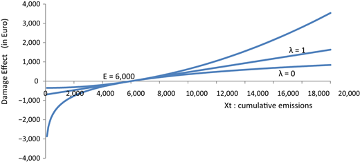
Numerous arguments concern the social damage functional form for climate change, and many approaches have been made since the dynamic integrated climate-economy (“DICE”) model of Nordhaus (1993). Even when using objective measurements, such as marginal temperature change, measurements of changes in human welfare remain quite subjective. For example, people who live in subtropical regions or islands and have been affected by rising sea levels will experience damage from increased carbon concentrations in the atmosphere. One could thus argue that damage should be modeled as an exponential function of global temperature or carbon concentration in the atmosphere. On the other hand, residents of Siberia would experience relatively less damage from climate change and may obtain benefits from warmer weather that would allow them to cultivate new types of crops that are otherwise vulnerable to cold weather. The welfare function would then be a linear or even logarithmic function of increased carbon concentration in the atmosphere. In short, there have been numerous arguments on what types of disasters would arise from increased temperatures and how this welfare can be measured numerically. Many of these ambiguous questions are not actually within the realm of economics. Even scientists disagree about these uncertain effects. Hence, this paper chooses the flexible Box-Cox transformation as the social damage function. We will leave this argument to be negotiated by policymakers, expecting them to make their decisions by choosing appropriate parameters as did Cassel and Mendelsohn (1985). The advantage of using Box-Cox is its flexibility, which allows us to model a welfare function while remaining indifferent about the form of the appropriate social damage function: this functional form can vary from a concave function such as log to a convex function such as quadratic. Figure 1 assumes the representative case of convex, linear and concave damage functions by choosing the different parameter λ to show the effects on permit prices of increasingly conservative views about the social damage produced by climate change: Equation 11 

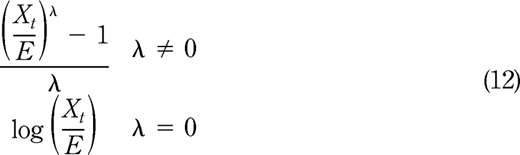
The Box-Cox transformation means that a different λ can characterize various climate change scenarios with different marginal damage effects on the atmosphere. As can be expected from the spot price equilibrium equation, whatever λ might be, the spot price surface is always higher than the spot price equilibrium without the environmental damage term. The damage from climate change always requires firms to pay more to obtain additional permits from the market. This shows the socially optimal price trajectory from the socially optimal emissions equilibrium. Using different λs, as seen in Figure 1, we can find socially optimum price paths of various climate change scenarios. From the concave to the convex function, numerous transformations of the social damage function can be chosen using the different perspectives of policymakers regarding climate change. The x-axis intercept of this flexible function is 1, so we need to change this to the emissions cap, E, of the compliance period. The modified function will be: Equation 12 

A reduced concentration of carbon in the atmosphere would slow down the global warming process. Much of this process, taking place in a black box, can be found in a number of scientific research projects, which is why we use the flexible damage function. In the Box-Cox transformation, the negative dependent variable represents negative damage: a positive effect on welfare (a slower global warming process or decreasing temperature) due to cumulative emissions being less than the cap. One major assumption in this modified Box-Cox damage function is that actual damage is driven by the difference in the level of emissions cap (e) that is artificially made by regulators. The actual damage level is determined by the gap between the level of emissions and the cap. The environmental regulator is assumed to set up an emissions cap considering the natural decaying rate of carbon or capacity for each period. Setting a cap at the zero-damage level reflects the regulator’s political will not to accelerate global warming or depress business activities. If regulators install stricter caps, then the economy would be depressed by severe environmental requirements, whereas a generous cap would result in failure to keep low carbon status, which would produce explicit monetary or implicit environmental losses in the near future. Figure 1 shows different transformations of the social damage function according to policymakers’ different perspectives to climate change. We assume that the damage is driven by the difference with the level of emissions cap and the actual cumulative emissions.

We now insert the Box-Cox damage function as social costs produced by climate change to the objective function. Equation (13) refers the value function as follows: Equation 13 

We followed the standard process for solving the stochastic optimality control problem. We use the principle of optimality for stochastic optimal control and characterize the value function in terms of the Bellman equation form[³].

Again, this optimal value of abatement not only optimizes the participating firm’s compliance costs but also maximizes social welfare by combining the environmental effects obtained from carbon emissions, as the Pigouvian tax does. We can characterize this optimal abatement as the socially preferred abatement level that represents both the representative firm and the environmental value that would be affected by climate change.

Next, by equating the marginal cost of the objective function and the spot price, we can obtain the spot price dynamics. The price is made by market players and not by anyone else (e.g. the government or other parties affected by climate change). On the other hand, the new spot price trajectory derived from the new objective function with the damage function considers the environmental effects. In equation (14), the spot price is equal to the marginal cost[⁴]: Equation 14 

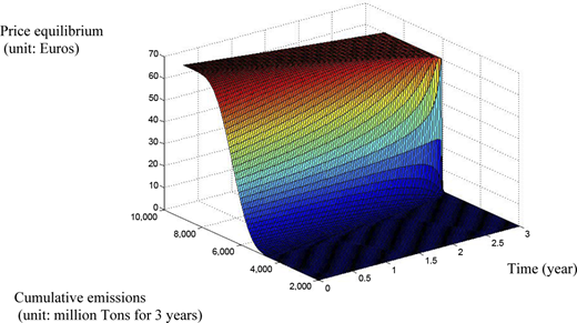
We define the total amount of banking and borrowing based on actual expected net cumulative emissions under the regulation cap. We can usually define the amount of banking if we have an excessive number of permits that exceeds the total number of permits that the government originally allowed. On the contrary, if net cumulative emissions exceed the original emissions allowance, the individual firm should borrow or purchase the number of permits from somewhere to cover the excess emissions. In equation (3), we defined R  _k as individual over-emissions at the period k. Hence, we now define R _k as a total amount of over-emissions that have an equivalent meaning with the net accumulative amount of borrowing (negative banking amount) during the period k. The sign of R _k is positive when net banking occurs and is negative when net borrowing occurs. This variable from banking and borrowing makes it possible to analyze the effect of the government’s regulations on the inter-temporal trading system. The optimized spot price path in Figure 2 is from the study by Seifert et al. (2008) defined by equation (15), assuming parameters in Table I: Equation 15 

This calibrated model uses the parameters found in Table I, which represents the EU-ETS as closely as possible. The penalty and the initial endowment of permits are given by Phase 1 of EU-ETS. The marginal abatement cost coefficient, c, and the volatility of market, σ, are from the study by Seifert et al. (2008). With the environmental weight, δ, it is assumed that the price trajectories pass through the expected price level of Phase 3 of EU-ETS (International Emissions Trading Associations, 2012, IETA).

The price path in Figure 2 describes how the price converges to the maximum level when the net expected cumulative emissions vary. During the initial period, the equilibrium price path exhibits a smoothly increasing shape. Once the representative agent knows whether the realized accumulative emissions are more than the emissions cap, the spot price approaches to zero or the maximum. Below-cap means that the price of obtaining a permit will be zero, but in the case of the price being above cap, the permit price will be almost the same as the present value of the penalty. We reinterpret this calibrated price trajectory as the one that only minimizes firms’ aggregated total compliance costs. The price equation considers only the market participant’s welfare in this case.

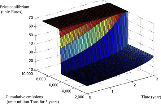
In comparison with the unrestricted model, Figure 3 illustrates the case of extremely restricted banking and borrowing. For example, even if there is net banking, it is worthless after this period. If the representative agent had borrowed a certain number of permits from the future, the firm has to pay that back with a high interest rate, which in fact is the same meaning as prohibitive borrowing. The simulation below illustrates a case where net banking has no value (100 per cent discount) in the future, and net borrowing should be paid back at three times of the original amount (i.e. at 300 per cent interest rate), which actually prohibits a borrowing scheme. When total emissions are less than the cap (net banking), the spot price is the same as the spot price when net banking is 0 because additional banking amounts do not contribute to lower prices later. When total emissions exceed the cap (net borrowing), the spot price hikes almost to the penalty level because the amount of borrowed permits that must be paid back later has almost tripled.

In this section, we apply different environmental damage scenarios characterized by the flexible Box-Cox functional form. Without considering environmental damage in carbon pricing, the market price would not be optimal from the social planner’s perspective. For example, an abatement that is too restrictive compared to the socially desired level would cause unnecessary compliance costs for participating firms, whereas excessively loose abatement requirements could produce relentless emissions due to the limited goals of each firm’s cost minimization behavior. Hence, the social planner has an incentive to match the actual emissions levels to the cap determined for each period. This goal can be achieved through manipulating the banking and borrowing system by matching emissions to the cap level for each period. Otherwise, free banking and the borrowing system might invalidate the emissions limitations in a certain period. Concentrated but legitimate emissions in certain periods of time, which were banked previously and borrowed from the future, can exceed the natural carbon decay level. This uneven emissions flow could invalidate the required cap for each period that is assumed to be socially desirable.

(Case 1) when λ = 2: quadratic damage function: pessimistic scenario.

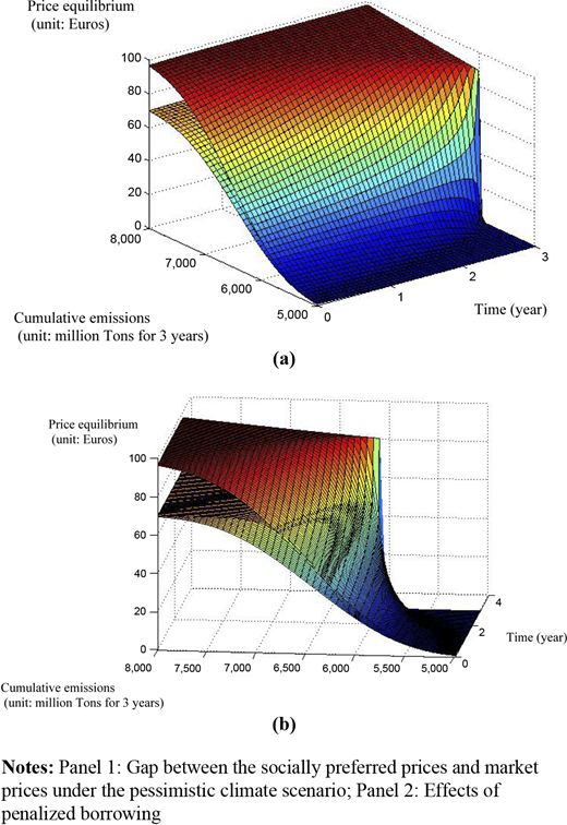
The marginally increasing social damage function can be called the pessimistic scenario for climate change. In other words, it also means that the marginal cost from the damage function also decreases as the abatement increases. In this case, we can predict that a regulatory authority would prevent excessive borrowing because of increasing damage but would not be very concerned about banking because of marginally decreasing abatement effects. Hence, the current use of permits by borrowing permits from the future should be limited reflecting the harmful effect of concentrated emissions during certain periods. This restriction is seriously needed in the case of net borrowing situations when the total amount of emissions exceeds the cap because net damage is positive. Regulations on borrowing can be modeled by a high discount rate on borrowed permits. For example, if 100 units of permits were borrowed from the future, only 80 permits would remain available for use; however, the company still has the obligation to pay back 100 units of permits instead of 80 units. The higher the discount rate, the less borrowing incentive is provided. In Figure 4, Panel 1 illustrates the gap between the socially preferred price path and original path. In Panel 2, the price trajectory in the middle shows the effect of a specific regulation on borrowing with a 70 per cent penalized increment in the future payback, which mitigates the gap of Panel 1.

In addition with a wider gap between the socially preferred price path and original one in Panel 1 of Figure 4 within the net borrowing range, there should be a major restriction on borrowing to let the market price path converge with the environment-friendly price path. The price discrepancy when a high amount of borrowing occurs refers to the fact that borrowing should be banned with a highly penalized borrowing regulation. The socially desired price path reflecting carbon prices that are higher than market prices represents regulated firms needing to have greater financial burdens than they would in free markets without environmental considerations. Of course, even if there is a penalty for borrowing permits, a firm has an incentive to borrow when a bull market on carbon is expected to persist until the next period.

On the contrary, within the net positive banking range, the gap between the original price and the newly optimized price path is not as wide, so putting a restriction on banking is not really needed. If discounting banked permits exists, for example, once the company banks 100 units of permits, then only 80 units are available during the next period. A small price discrepancy means that a small regulation on banking with a moderate discount rate is needed.

Therefore, in this pessimistic case, we can conclude that the banking rule can be comparatively generous from the slight difference of the price path, but the borrowing rule will be restrictive regarding the narrowing the price gap in this pessimistic case. Panel 2 of Figure 4 provides an example of a specific borrowing regulation with 70 per cent penalized increments in future paybacks and no penalized discounting on banking.

(Case 2) when λ = 0: logarithmic damage function: optimistic scenario.

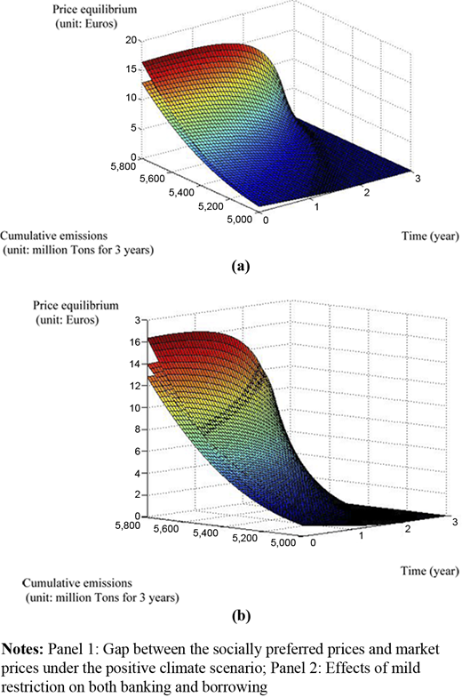
This scenario describes a positive situation concerning climate change from the diminishing marginal effect of accumulated carbon. This damage function means a marginally increasing abatement effect. Hence, the marginal cost driven by the damage function could be infinitely high enough when the accumulated amount of emissions is low or close to zero (net banking). On the other hand, the marginal cost decreases when the accumulation is relatively high (net borrowing). In this case, the regulatory authorities would be incentivized to prohibit excessive banking due to less effective abatement outcomes, whereas they would have less incentive to restrict borrowing because of its low marginal costs. Therefore, banking should be regulated with a high discount rate of banked permits.

In the pessimistic scenario described in Figure 5, Panel 1 highlights the necessity for banking restrictions as shown in the wide price discrepancy within the net banking interval. Panel 2 illustrates the effect of a comparatively generous borrowing rule and a restrictive banking rule.

Within the net banking range, the discrepancy between the socially preferred price path and the original one in Panel 1 of Figure 5 is larger than the pessimistic case. If the gap is large in the banking range in the extreme situation, it means that banking should be abandoned, which means 100 per cent discounted banking. Therefore, there should be a restriction on banking to converge with the environment-friendly price path. If a firm cannot expect higher capital gain by banking permits for future use, they may try to exhaust permits within this compliance period.

In comparison, in the net borrowing range, the gap between the original price and the newly optimized price path is not as wide as the pessimistic scenario, so there is little reason to put restrictions on borrowing. This optimistic case allows us to conclude that the borrowing rule can be comparatively generous due to the small difference in the price path, but the banking rule can be more restrictive for filling the gap, as shown Panel 2 of Figure 5.

(Case 3) when λ = 1: linear damage function: neutral scenario.

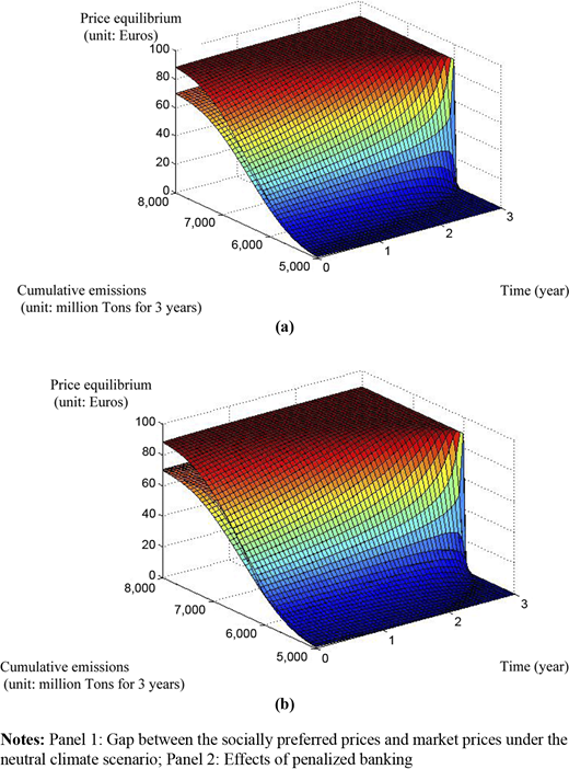
The effect of the neutral scenario requires a mixture of the pessimistic and optimistic cases. In the case of positive banking, the socially desirable price path is slightly higher than the market price path because original price is relatively close to 0 as seen at Panel 1 of Figure 6. The social planner does not need to have restrictions on banking; a small discount rate is sufficient for getting closer to the social optimum price path. In a neutral scenario, Panel 1 suggests that a banking restriction is not needed due to a narrow price gap. Panel 2 shows that a borrowing restriction can narrow the price gap when cumulative emissions are greater than the cap.

In the case of net borrowing, the gap in Panel 2 of Figure 6 is relatively higher than the case for net banking in Panel 1 of Figure 6. We can thus say that social planners can achieve the optimum price level by imposing a more restrictive borrowing rule than in the net banking case. This is normal in most actual markets because putting a regulation on banking would result in bigger emissions exhausting permits. Borrowing has usually been prohibited in many actual markets such as the second period of EU-ETS or SO₂ market in the USA.

In general, industries prefer to relax regulations, allowing banking and borrowing rules to be determined politically by stakeholders. In addition, past studies on banking and borrowing rules with respect to the cap-and-trade system commonly conclude that adding this flexibility to permit transactions will improve the total welfare of market participants. Hoarding permits until market prices rise in the future or exhausting permits before market prices go down produce efficiencies by arbitraging from the past to the future

There is a tradeoff, however, between environmental objectives and market outcomes. The more freedom firms have, the more likely the actual price trajectory will be far from the socially desirable one. Hence, the social planner can harmonize the interests of regulated firms and environmental goals by incorporating the environmental damage effect into the pricing model, which enables the social planner to adjust the banking and borrowing regulation. Some markets such as California AB 32 or Phase 2 of the EU-ETS typically completely prohibit a borrowing. During the first period of the EU ETS market, banking was prohibited because it can induce firms to reduce their gas emissions more, and sometimes banking is not the optimal way to maximize social welfare.

Hence, this paper departs from previous studies in that we allow policymakers to choose policy tools in a more sophisticated manner. In addition, we model for price calibration that enables us to use inter-temporal permit trading regulation to mimic a socially desirable price trajectory. Based on the policymaker’s model choice, we can roughly expect the type of policy combination (i.e. restriction or incentives on banking or borrowing) and the levels of restriction that are needed. The benchmark gained from this model can provide supporting evidence for modifying inter-temporal regulation.

This study has some limitations, however. While it uses the Box-Cox transformation to describe the unknown type of damage function regarding climate change, it does not cover every possible global warming effect. The socially desirable price path was modified from the original price path by the environmental damage term and may not be the simple replacement we used in this paper using the Box-Cox transformation. Furthermore, when the damage function is more complicated than what we are able to express, various policy combinations with restrictions on both borrowing and banking may be needed.