


Changing climate has increasingly become a challenge for smallholder farmers. Identification of technical, institutional and policy interventions as coping and adaptation strategies and exploring risks of their adoption for smallholder farms are the important areas to consider. The aim of the present study was to carry out an in-depth analysis of adaptation strategies followed and the associated risk premium in technology adoption.
The study was carried out in the dryland systems of three Indian states – Andhra Pradesh, Karnataka and Rajasthan – and was based on a survey of 1,019 households in 2013. The flexible moment-based approach was used for estimating the stochastic production function, which allowed estimation of the relative risk premium that farmers are willing to pay while adopting the technologies to avoid crop production risks.
In all the three states, the risk premium (INR ha−1) was higher for farm mechanization compared to supplemental irrigation, except in the case of Andhra Pradesh. The higher the level of technology adoption, the higher the risk premium that households have to pay. This can be estimated by the higher investment needed to build infrastructure for farm mechanization and supplemental irrigation in the regions. The key determinants of technology adoption in the context of smallholder farmers were climatic shocks, investment in farm infrastructure, location of the farm, farm size, household health status, level of education, married years, expected profit and livestock ownership.
Quantification of the risk premium in technology adoption and conducting associated awareness programs for farmers and decision-makers are important to strengthen evidence-based adoption decisions in the dryland systems of India.
1. Introduction
Agriculture, in general, is very much affected by climate change and variability. Climate change projections for India up to 2100 indicate that there will be an increase in temperature by 2-4°C with no substantial change in precipitation (Kavikumar, 2010). This increase will be higher in the dryland production systems. Climate change not only affects the mean yield of crops but also induces variability in yield (Palanisami et al., 2014). These research findings substantiate the hypothesis that rain-fed farming will be severely affected by climate change and variability. Although rain-fed crops can tolerate high temperatures, crops grown during the post-rainy (Rabi[1]) season are vulnerable to changes with minimum temperature (Venkateswarlu and Rama Rao, 2010). This also has strong implications for livestock feed quality and quantity and thus to their productivity, as crop residues constitute major feed components in South Asia, generally.
Therefore, it is important to have strategies in place that can help farmers cope with these uncertainties and vulnerability. These strategies can involve a variety of interventions, e.g. technical, institutional or policy. In this context, a household-level vulnerability analysis could provide a basis on which interventions can be identified and targeted to respective households (Palanisami et al., 2015). More generally, vulnerability analysis will be a key component of the theory of change, as it provides a basis on which interventions can be targeted and assessed on households and communities in the context of overall livelihood strategies and the biophysical characteristics of the production system.
There are not many opportunities available to increase agricultural production by expanding the crop area. Even under a climate change scenario, agricultural intensification using technology as an option to increase productivity seems possible, due to the availability of a number of suitable agricultural technologies. However, the current level of technology adoption is comparatively low, and the increasing uptake of technology use will be a major task ahead, as it involves interaction of both farm- and policy-level interfaces. There could be a number of constraints to technology adoption, such as the cost of technology, suitability of technology depending on the farmers’ needs and the high risks involved, among others. Identifying such risks and determinants of technology adoption will contribute to agricultural intensification efforts (Espinoza, 2012; Kassie et al., 2008; Juma et al., 2010). Thus, this paper provides evidence of how determinants of risk and the risk premium associated with technology adoption could be identified and addressed through policy interventions in India. Therefore, the main objective of this study is to examine the factors and risks associated with technology adoption. It provides an in-depth analysis of the identification of agricultural water management technologies and quantification of risk in adopting these technologies by smallholder farmers.
2. Materials and methods
2.1 Location of the study regions
The study region was selected from the Dryland Production System in South Asia of the CGIAR Research Program (CRP). The selection was based on systematic overlaying of data, such as aridity index, length of growing period (<90 days, <180 days), land use and land cover and resource degradation (Haileslassie et al., 2016). Three regions/states (Andhra Pradesh, Karnataka and Rajasthan in India) were selected for the study. Six districts – Barmer, Jodhpur and Jaisalmer in west Rajasthan, Bijapur in Karnataka and Kurnool and Anantapur in Andhra Pradesh – were selected representing different degrees of vulnerability and potential for agricultural intensification. Figure 1 shows the location map of the study region and the target districts.
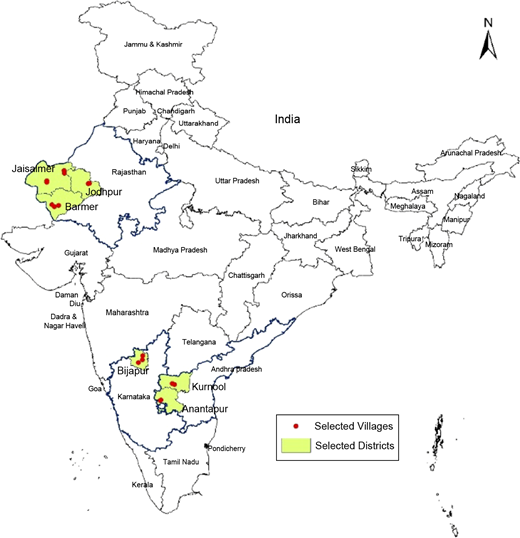
In terms of production systems, Rajasthan purposely includes low-rainfall rangelands where pastoral and agro-pastoral systems predominate. Elsewhere in India, areas with sustainable intensification are dominant, except for a large vulnerable area in peninsular India centered on parts of Maharashtra, Andhra Pradesh and Karnataka. In all three states, mixed crop–livestock systems are predominant (Haileslassie et al., 2013, 2016). In these mixed crop–livestock systems, one of the major determinants of agricultural production is the soil type. Two major soil types can be identified: red soil- (Alfisols, Acrisols and Entisols) and black clayey soil (Vertisols)-based systems (Haileslassie et al., 2013, 2016). Red soils make up 60-65 per cent of the cropping belt in South India (e.g. Anantapur and Kurnool districts in Andhra Pradesh) followed by black soils (e.g. Bijapur in Karnataka) (Table I).
Sample states, target districts, major production systems and distribution of sample farm households
| Study regions and target districts | Subdistrict (Mandala/Tehsil/Taluk/Block) | Key production system | No. of sample farmers surveyed |
|---|---|---|---|
| Anantapur and Kurnool (Andhra Pradesh) | Kalyandurg, Dhone | Mixed crop-livestock, red (and black) soils | 513 |
| Bijapur (Karnataka) | Bijapur | Mixed crop-livestock, black soils | 250 |
| Jodhpur, Barmer and Jaisalmer (Rajasthan) | Osian, Chohtan, Jaisalmer | Rangeland, agro-pastoral | 256 |
Note:
Depending on the location, Mandal/Tehsil/Taluk/Block represent the second lower administrative units in India
Data were collected from the households during the 2013 production season using a pretested interview schedule. The people entrusted with the task of collecting data were trained in the data collection process and description of variables. Focus group discussions were held in the selected villages at the beginning of the survey to introduce the concepts of the research study, and to also get first-hand information about the village profile, climate shocks and adaptation strategies followed. A total of 1,019 farmers were surveyed (Table I). The collected data set includes household characteristics – farm size, household size, distance to market for sales, gender, household education, household age, household marital status, household married years, number of earning male and female members, health status, experience in farming, number of visits made by farmers to extension officials, number of visits made by extension officials to farmers, occurrence of extreme climate events such as droughts and hailstorms, irregular weather, untimely rain, animal disease, livestock ownership, possession of skill development activities, changes in crop pattern, change in planting dates, change in crop production practices, sale of livestock, borrowing money, relying on assistance from the government, investment in farm machinery, investment in infrastructure, crops grown in each season (Rabi and Kharif), quantities and costs of inputs (such as seed, fertilizer, labor, bullock and machine power, fuel and electricity), main and secondary products (e.g. crop residues) outputs, etc. Information on the type of technologies adopted by farmers and the costs and benefits of using these technologies were also collected. Because technology adoption and input use largely depend on location, the analysis was carried out separately for Andhra Pradesh, Karnataka and Rajasthan study sites.
2.2 Framework to quantify risk in technology adoption and empirical studies
2.2.1 Quantification of risk in technology adoption.
A number of studies have been conducted on production risk and farm technology adoption. The stochastic production models are used to estimate the effect of input choice on production risk. For example, Just and Pope (1978) provided a general stochastic specification of the production function. This model includes two general functions – one for the mean output and the other for the variance in production. The two functions can be used to study the effects of inputs/technologies on the mean and variance in production. The model allows inputs/technologies to be either risk-increasing or risk-decreasing. If the marginal contribution of an input to variance is positive then the input is risk-increasing, otherwise, it is risk decreasing. Although this model is a good generalization of stochastic specification models, it does not restrict the effects of inputs on the variance to be related to the mean. To alleviate this shortcoming, Antle (1983, 1987) proposed a moment-based approach and showed that the mean input restricts the effects of inputs across the second and higher moments. The moment-based approach allows more flexible representation of input distribution and allows for the identification of risk parameters.
The procedure proposed by Antle (1983, 1987) is an “nth” degree approximation to a stochastic variable such as profit distribution. It is obtained by estimating the “nth” degree polynomial whose coefficients are functions of the first “n” moments of the distribution. Coefficients of the polynomial model are estimated using generalized least squares (GLS). The estimators have desirable asymptotic statistical properties. Additionally, if the random variable under study has a finite range, the set of moments uniquely defines the probability density function. So, this moment-based approach is quite flexible and has a sound statistical foundation. The general model is described below.
2.2.1.1 General model.
Let us assume that farmers in a region grow a single crop (with output denoted by q), say groundnut, using many inputs, X = (x1,x2…xn). Also assume that the farmers are risk-averse. The output production function is given by f(X;S;β), where S is a vector of extra shifters, including farmer-specific characteristics (such as age, experience, household size engaged in farming, etc). and farm-specific characteristics (such as plot size, technology adopted, etc.), and β is a vector of parameters to be estimated which are assumed to satisfy the regularity conditions: continuous with respect to all variables and twice differentiable. The output unit price is denoted by p, and the input prices are given by the vector r = (r1,r2,…rn). We assume that the prices of output and inputs are deterministic, whereas the output q is a random variable depending on factors over which the farmer has no control. This risk in crop output, denoted by ε, is assumed to have a distribution denoted byG(.). Also, the function f is assumed to be continuous and twice differentiable. Farmers in rain-fed areas face uncertainty over the availability of inputs such as timely labor and supplemental irrigation. They depend on machine labor and supplemental irrigation sources, the supplies of which are uncertain. Hence, the output is also uncertain. The profit function of the farmer is given by equation (1):
Because the output is a random variable, equation (1) implies that the profit Π is also a random variable, and it is assumed that the expected value is finite. If the farmer is risk-neutral, then his objective will be to maximize his expected profit. He will be indifferent to the variance, that is risk, in profit. However, if he is risk-averse, which the authors assume, he wants to maximize the expected utility of profit. So, his problem can be stated mathematically as depicted below in equation (2):
Where:
U(.) is the Von Neumann–Morgenstern utility function that represents the risk preferences of the farmer. The farmer will prefer to maximize E(U(Π)) with respect to the input, Xw, supplemental irrigation water. The first-order condition for optimal use of input, say supplemental irrigation water,Xw, is given by equation (3):
Where:
U′ = ∂U(Π)/∂Π is a derivative of utility with respect to income. For risk-neutral farmers who will maximize their expected profit, the ratio of input price over output price, that is (rw/p), will be equal to the expected marginal contribution of input xwto profit function f(X;S;β). So, for these farmers, the second term on the right-hand side of equation (3) will be zero, and for risk-averse farmers, it will be non-zero.
2.2.1.2 Flexible moment model.
In principle, equation (3) can be solved to obtain the optimum level of Xw. The optimal solution would depend on the prices of supplemental irrigation, inputs, output and the shape of functions U(.), f (.) and G(.), which are usually unknown. Hence, this problem is empirically difficult. In addition to the choice of technology specification, the distribution of ε needs to be known and the farmer’s preferences need to be specified. For this reason, Antle (1983, 1987) proposed a flexible estimation approach that has the advantage of requiring only cross-sectional information on prices and input quantities. The important feature of this approach is that the solution to the producer problem can be written as a function of input levels alone. According to the approach, maximizing the expected utility of profit with respect to any input is equivalent to maximizing a function of moments of the distribution of ε, those moments having themselves the input vector X as an argument. This is given by equation (4):
Where μj is the jth moment of the farm profit and F(.) is the cumulative distribution function completely unspecified. Using the first-order condition, it can be shown that the marginal impact of kth input on the first moment is given by equation (5):
Where:
represents the “weight” attributed by the farmer to the jth moment of the profit distribution. The analysis is carried out technology by technology, because each technology contributes in a different manner to the moments of the profit distribution. Thus, for each technology, the following model was estimated [equations (7) and (8)]:
Where:
The model [equation (7)] has two important features. The first is that it shows that the marginal contribution of an input (technology) to the first moment is a linear function of marginal contribution of the input to the second (i.e. variance: ∂μ2(X)/∂xk), third (i.e. skewness: ∂μ3(X)/∂xk) and other higher moments. A negative sign on the marginal contribution of an input (i.e. the variance) to the second moment indicates that the input is risk-reducing, while a positive sign indicates that it is risk-increasing. Similarly, a negative sign on the marginal contribution of an input to the third moment implies that the input is a downside (DS) risk-increasing function, and a positive sign means that the input is a DS risk-decreasing function. Researchers usually take up to the third moment (i.e.m = 3) because the second moment represents variance (i.e. risk) and the third moment represents skewness, and usually higher moments have less influence on the profit.
2.2.1.3 Risk premium estimation.
The Arrow–Pratt (AP) absolute risk-aversion coefficient is defined by equation (9):
Using equations (6) and (8) in (9), APk = 2θ2k. Similarly, the DS risk-aversion measure is as given by equation (10):
Therefore, using equations (6) and (8) in (10), DSk = −6θ3k . Thus, the parameters θ2k and θ3k can be directly interpreted as the AP and DS risk coefficients, respectively. They can be interpreted as a marginal contribution of each moment to risk premium (Groom et al., 2008), which is defined as the difference between a guaranteed or a certain income and a risky income that generates the same level of utility. Risk premium is the amount of income that a risk-averse farmer is willing to pay to avoid the risk associated with technology adoption. Assuming that the farmer is concerned only with the first three moments of profit distribution, the risk premium is given by equation (11):
Where:
μ2 and μ3 are the measures for the second and third moments, respectively, of the profit for an individual farmer.
A positive value for the AP coefficient means that the farmer is risk-averse. This denotes that they are willing to forego a proportion of their expected profit to avoid the risk associated with the technology adopted. Similarly, a positive value for DS risk means that the farmer is averse to the DS risk. This highlights that they are risk-averse to a negatively skewed profit distribution. A positive value for risk premium, i.e. RP > 0, means that the farmer has a positive willingness to pay to be insured against risk. The constant term θ1k should be non-significant. If this is positive and significant, it implies that the particular input is overused. If this is negative and significant, it implies that the particular input is underused. The framework of the analysis is given in Figure 2.
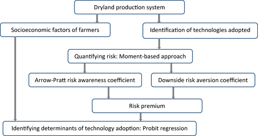
Framework of the model showing the links between technology adoption and risk premium calculations
Framework of the model showing the links between technology adoption and risk premium calculations
2.2.2 Empirical studies.
Many researchers applied the approach proposed by Antle (1983, 1987) to quantify risk in production, and some referred to it for study purposes. Espinoza (2012) studied the potato production risk and irrigation technology adoption among farmers in Chile. The results indicated that education level, proportion of land under secure tenure arrangements, access to credit and knowledge from extension activities are determinants of irrigation technology adoption. Using the moment-based approach of Antle (1983, 1987), Yesuf and Bluffstone (2009) investigated the impacts of the adoption of chemical fertilizer use, and soil and water conservation technologies on production risks. They found that adoption of chemical fertilizer use reduces yield variability, but it increases the risk of crop failure, and adoption of soil and water conservation technologies has no impact on yield variability, but it reduces the DS risk of crop failure. Juma et al. (2010) explored the production risk and farm technology adoption in rain-fed, semiarid lands of Kenya. Their study showed that yield variability and the risk of crop failure affect technology adoption decisions.
Kassie et al. (2008) examined the role of production risk in sustainable land management technology adoption in Ethiopia. The study identified that the impact of production risk varied by technology type. Production risks, which were measured by the second and third moments, had a significant impact on the adoption of fertilizer use and extent of adoption. Koundouri et al. (2003) derived the conditions under which a risk-averse farmer with incomplete information adopted an efficient irrigation technology to hedge against production risk. They found that the higher the expected profit, the greater the probability of farmers adopting a new irrigation technology. Similarly, higher the variance of profit, greater will be the probability to adopt new irrigation technologies to save water and reduce production risk. Shajari and Bakhshoodeh (2006) studied the link between new seed varieties and wheat production risk in Iran using a moment-based approach, and showed that new seed varieties are risk-increasing with higher cost of risk. They concluded that, the more risk-averse farmers are, the less likely they are to adopt new seed varieties to decrease production risk.
2.2.3 Model execution.
Even though several approaches are available to address technology adoption and risk assessment, this paper follows the flexible, moment-based approach outlined by Antle (1983, 1987). The methodology has two stages and has been followed by many authors (Groom et al., 2008; Shajari and Bakhshoodeh, 2006; Espinoza, 2012). The advantage of this method is that it takes into account both variability and skewness in the yield. Initially, three moments of the profit and risk-aversion coefficients, and the risk premium are computed. In Step 1, total observed profit per hectare is regressed at all levels, squared and cross-products of all inputs. This indicates the selection of linear quadratic form, because it is a good second-order approximation of the profit function (Kumbhakar and Tveterås, 2003). In Step 2, residuals of the fitted regression are used to compute conditional higher moments (variance and skewness), and are regressed at all levels, squared and cross-products of inputs. This approach was used in many studies (Antle, 1983; Kim and Chavas, 2003; Koundouri et al., 2003). Mathematical expressions for derivatives of these moments in relation to each input are then computed. Finally, using these derivatives for individual farmers, equation (7) above was estimated through a two-stage, least squares regression analysis. The instrumental variables used for this purpose are:
distance of the farm from the market for disposal of the outputs;
investment in farm machinery;
investment in new infrastructure; and
awareness of technologies (dummy variable).
After estimating equation (7), the AP risk-aversion coefficient and DS risk coefficient are computed, and they are substituted in equation (11) to estimate the risk premiums. Then, the relative risk premium is computed by dividing the risk premium by the expected profit.
To identify the determinants of adoption of a technology by farmers, the socioeconomic characteristics of the farmer along with the relative risk premium are then used in a probit regression model (with the dependent variable being a binary variable taking the value 1 for those farmers who adopted a particular farming technology and 0 for those who have not adopted it).
3. Results and discussion
3.1 Socioeconomic profile of households
The descriptive statistics of variables used in this study for the three locations are provided in Table II. The farm size ranges from 2.22 to 3.67 ha in the sample. Similarly, household size ranges from 4.38 to 5.54. Farmers in Andhra Pradesh travel, on average, 6.5 km to sell their farm output. These distances for farmers in Karnataka and Rajasthan were 31.0 and 12.4 km, respectively. In all the locations, about 89 to 96 per cent of the study households had male heads. The mean age of the household head from all the states is about 50 years and they are poorly educated. Farmers have 22 to 32 years of experience in agricultural production. Farmers in the three states had experienced different combinations of shocks, which were included as dummy variables in the analysis. In Rajasthan, 99 per cent of the farmers owned livestock, because it was the major component of farm income. In Andhra Pradesh and Karnataka, 54 and 40 per cent of the farmers, respectively, owned livestock. The farmers had used several farm-level adaptation strategies, such as possessing livestock, small farm mechanization, providing supplemental irrigation, change in cropping pattern and planting dates and developing skills in technology adoption through training. However, only the major strategies were included in the model by using dummy variables for each of the strategies (Table II for more details).
Descriptive statistics of variables used in the modelling of farm technology adoption
| Dependent variable | Andhra Pradesh | Karnataka | Rajasthan | Description | |||
|---|---|---|---|---|---|---|---|
| Mean | SD | Mean | SD | Mean | SD | ||
| Profit (INR ha−1) | 19,676 | 37,435 | 70,538 | 68,398 | 38,713 | 50,403 | Continuous |
| Household age (years) | 47.81 | 13.47 | 51.80 | 13.02 | 50.79 | 13.68 | Continuous |
| Gender | 0.96 | 0.19 | 0.94 | 0.25 | 0.89 | 0.31 | D.V. = 1 for male and 0 for female |
| Household education | 1.56 | 1.01 | 1.70 | 1.08 | 1.43 | 0.69 | Discrete with seven-point scale, with 1 for no formal education and 7 for postgraduate education |
| Household marital status | 0.97 | 0.16 | 0.96 | 0.20 | 0.86 | 0.35 | D.V. = 1 if married and 0 otherwise |
| Household married years | 27.39 | 14.59 | 29.62 | 13.89 | 30.32 | 15.99 | Continuous |
| Household size | 4.38 | 2.00 | 5.54 | 2.63 | 5.48 | 2.54 | Continuous |
| Experience in farming (years) | 24.14 | 12.37 | 22.40 | 12.01 | 32.27 | 15.05 | Continuous |
| Earning male members | 1.88 | 1.12 | 1.58 | 0.70 | 1.73 | 1.15 | Continuous |
| Earning female members | 1.69 | 1.00 | 1.28 | 0.65 | 0.77 | 1.04 | Continuous |
| Health status | 1.53 | 0.94 | 1.42 | 0.65 | 1.80 | 1.29 | Discrete with six-point scale, 1 for good and can perform agricultural activities and 6 for bad |
| Farm size (ha) | 2.22 | 2.50 | 3.67 | 4.82 | 2.64 | 3.08 | Continuous |
| Livestock ownership | 0.54 | 0.50 | 0.40 | 0.49 | 0.99 | 0.09 | D.V. = 1 if owns livestock and 0 otherwise |
| Distance to market for sales (km) | 6.48 | 30.81 | 31.03 | 17.03 | 12.43 | 9.88 | Continuous |
| Number of visits made by farmers to extension officials | 2.19 | 1.16 | 2.26 | 0.58 | –a | –b | Discrete |
| Number of visits made by extension officials to farmers | 2.52 | 1.34 | 0.84 | 0.73 | – | – | Discrete |
| SC1AP | 0.30 | 0.46 | D.V. = 1 if drought, hailstorm and irregular weather are encountered and 0 otherwise | ||||
| SC2AP | 0.22 | 0.41 | D.V. = 1 if drought alone is encountered and 0 otherwise | ||||
| SC3AP | 0.04 | 0.20 | D.V. = 1 if drought, untimely rain and irregular weather are encountered and 0 otherwise | ||||
| SC4AP | 0.06 | 0.23 | D.V. = 1 if drought, animal disease, untimely rain and irregular weather are encountered and 0 otherwise | ||||
| SC1KA | 0.33 | 0.47 | D.V. = 1 if drought, untimely rain and irregular weather are encountered and 0 otherwise | ||||
| SC2KA | 0.16 | 0.37 | D.V. = 1 if drought, animal disease, untimely rain and irregular weather are encountered and 0 otherwise | ||||
| SC3KA | 0.16 | 0.37 | D.V. = 1 if drought and untimely rain are encountered and 0 otherwise | ||||
| SC1R | 0.22 | 0.41 | D.V. = 1 if all the shocks except for floods are encountered and 0 otherwise | ||||
| SC2R | 0.18 | 0.38 | D.V. = 1 if all the shocks except for floods and low temperature fluctuations are encountered and 0 otherwise | ||||
| SC3R | 0.11 | 0.32 | D.V. = 1 if the shocks drought, hailstorm, animal disease and untimely rain are encountered and 0 otherwise | ||||
| cfaig | 0.18 | 0.38 | 0.82 | 0.39 | D.V. = 1 if they possess skill development activities, 0 otherwise | ||
| cfccp | 0.20 | 0.40 | 0.56 | 0.50 | D.V. = 1 if a change in cropping pattern is followed as a coping strategy and 0 otherwise | ||
| cfcpd | 0.12 | 0.33 | 0.43 | 0.50 | D.V. = 1 if a change in planting date is followed as a coping strategy and 0 otherwise | ||
| cfic | 0.09 | 0.29 | 0.24 | 0.43 | D.V. = 1 if improved crop production practices are followed and 0 otherwise | ||
| cpsi | 0.10 | 0.30 | D.V. = 1 if supplemental irrigation is provided and 0 otherwise | ||||
| cfsls | 0.18 | 0.39 | 0.48 | 0.50 | D.V. = 1 if livestock is sold as a coping strategy and 0 otherwise | ||
| cnfbm | 0.87 | 0.34 | 0.87 | 0.34 | 0.75 | 0.43 | D.V. = 1 if money was borrowed from relatives/friends and 0 otherwise |
| cnfrag | 0.36 | 0.48 | 0.76 | 0.43 | 0.46 | 0.50 | D.V. = 1 if relying on assistance from the government and 0 otherwise |
| cnfomc | 0.66 | 0.48 | D.V. = 1 if out-migration to cities is used as a coping strategy and 0 otherwise | ||||
| cflf | 0.52 | 0.50 | D.V. = 1 if land is left fallow and 0 otherwise | ||||
| cfmpoultry | 0.17 | 0.38 | D.V. = 1 if possessing poultry and goats is used as a farm-based coping strategy and 0 otherwise | ||||
| cnfsnfe | 0.63 | 0.48 | D.V. = 1 if shifting to non-farm employment is used as a non-farm-based coping strategy and 0 otherwise | ||||
| cnflfc | 0.36 | 0.48 | D.V. = 1 if there is less food consumption or a change in eating habits is used as a coping strategy and 0 otherwise | ||||
| Investment in farm machinery (INR) | 24,765 | 18,421 | 14,004 | 24,551 | 47,517 | 138,323 | Continuous |
| Investment in infrastructures (INR) | 15,582 | 42,103 | 100,893 | 63,651 | 48,257 | 160,547 | Continuous |
Notes:
SC1AP: Climate shock scenario 1 for Andhra Pradesh, SC2AP: Climate shock scenario 2 for Andhra Pradesh, SC3AP: Climate shock scenario 3 for Andhra Pradesh, SC4AP: Climate shock scenario 4 for Andhra Pradesh, SC1KA: Climate shock scenario 1 for Karnataka, SC2KA: Climate shock scenario 2 for Karnataka, SC3KA: Climate shock scenario 3 for Karnataka, SC1R: Climate shock scenario 1 for Rajasthan, SC2R: Climate shock scenario 2 for Rajasthan, SC3R: Climate shock scenario 3 for Rajasthan, cfaig: Possession of skill development activities, cfccp: Change in cropping pattern, cfcpd: Change in planting date, cfic: Change in crop production practices, cpsi: Invest in supplemental irrigation, cfsls: Sale of livestock, cnfbm: Borrowing of money, cnfrag: Assistance from government, cnfomc: Out-migration to cities, cflf: Left land fallow, cfmpoultry: Possessing poultry and goats, cnfsnfe: Shifting to non-farm employment, cnflfc: change in food consumption/eating habits. D.V. = dummy variable; SD = Standard Deviation;
In Rajasthan, 219 farmers did not visit any extension official;
In Rajasthan, extension officials did not visit 226 farmers; USD 1 = INR 65
Focus group discussions held with the farmers had indicated that they were facing problems in the adoption of small farm mechanization and in providing supplemental irrigation, because of the high cost and frequency of use in crop production. In the case of possession of livestock and change in cropping pattern, they did not face any challenges. Hence, in the analysis of technology adoption and risk, only small farm mechanization and supplemental irrigation strategies were included.
Among the different adaptation strategies, farm mechanization is commonly followed in all the three regions even though it is comparatively costly. Similarly, providing supplemental irrigation is another technology that is used mostly by rain-fed farmers of Andhra Pradesh and Karnataka (Figure 3). The two technologies are adopted in all the three regions, and it is assumed that the constraints to overall technology adoption will be captured when analyzing the adoption of these two technologies.
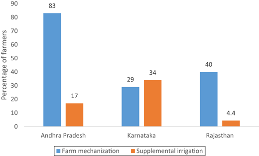
Prominent technologies/adaptation strategies followed by farmers in the study region
Prominent technologies/adaptation strategies followed by farmers in the study region
A high income can be earned by adopting technologies. However, the level of adoption of these technologies is comparatively low, and this may be because of the inherent risk associated with the adoption of new practices that derives mainly from uncertainty of future income flows. Therefore, it is important to identify how the cost of this risk or uncertainty (otherwise referred to as “premium”) varies across the adoption of different technologies. Several studies dealing with rain-fed agriculture also indicated that risk is an important determinant of technology adoption. For example, Maurice et al. (2010) identified that factors such as yield variability and risk of crop failure affect technology adoption decisions in the rain-fed, semiarid lands of Kenya. As stated by Maurice et al. (2010), only economically secure farmers who have sufficient defense against DS risk will undertake profitable investments and innovations, while most of the poor remain caught in a risk-induced poverty trap (Mosley and Verschoor, 2005; Yesuf and Bluffstone, 2009).
3.2 Estimation of parameters on the adoption of technologies using moment-based models
As stated in Section 2, a quadratic form of functional relationship between net revenue per hectare and the five inputs (seed, fertilizer, labor, use of machine labor [small farm mechanization] and irrigation water [supplemental irrigation]) was fitted. The moment functions were estimated according to the methodology stated in Section 2. The estimated coefficients of the quadratic form of the first three moments are presented in Tables III, IV and V for Andhra Pradesh, Karnataka and Rajasthan, respectively.
Estimates of parameters of three moments of profit function for Andhra Pradesh
| Variable | First moment | Second moment | Third moment | |||
|---|---|---|---|---|---|---|
| Coefficient | t-value | Coefficient | t-value | Coefficient | t-value | |
| Constant | 0.2788** | 2.0792 | −0.4496 | −1.5259 | −2.0756* | −1.7168 |
| Seed (kg/ha) | 0.1393 | 1.4030 | 0.7023*** | 3.2192 | 3.4935*** | 3.9030 |
| Fert (kg/ha) | −0.3097*** | −3.0295 | −0.3001 | −1.3359 | −1.9205** | −2.0833 |
| HBLB (number of days/ha) | 0.0638 | 0.6854 | 0.5925*** | 2.8943 | 2.4376*** | 2.9023 |
| MCLB (number of days/ha) | −0.1154 | −1.3267 | −0.3964** | −2.0743 | −1.4561* | −1.8569 |
| Water (m3//ha) | 0.5800*** | 4.0614 | 0.8671*** | 2.7624 | 2.0762 | 1.6122 |
| Seed2 | 0.2587*** | 6.9485 | 0.1677** | 2.0491 | 0.1939 | 0.5774 |
| Seed × Fert | −0.1307*** | −2.3637 | −0.1225 | −1.0076 | −0.6524 | −1.3082 |
| Seed × HBLB | −0.0969*** | −2.3758 | −0.2855*** | −3.1833 | −1.2143*** | −3.3005 |
| Seed × MCLB | −0.0004 | −0.0074 | −0.0963 | −0.9190 | −0.1612 | −0.3750 |
| Seed × Water | −0.2173*** | −4.1520 | −0.0161 | −0.1404 | 0.5427 | 1.1500 |
| Fert2 | 0.0051 | 0.2234 | 0.0365 | 0.7327 | 0.3137 | 1.5333 |
| Fert × HBLB | 0.1354*** | 2.9392 | 0.0036 | 0.0358 | 0.1693 | 0.4076 |
| Fert × MCLB | 0.0829 | 1.5301 | 0.1298 | 1.0902 | 0.4886 | 0.9998 |
| Fert × Water | 0.0907** | 2.2873 | −0.0199 | −0.2281 | −0.3726 | −1.0422 |
| HBLB2 | −0.0145 | −0.7021 | −0.1074*** | −2.3707 | −0.4444*** | −2.3916 |
| HBLB × MCLB | −0.0140 | −0.4388 | 0.1461** | 2.0856 | 0.4824* | 1.6790 |
| HBLB × Water | 0.0624 | 1.4673 | 0.2473*** | 2.6465 | 1.1269*** | 2.9394 |
| MCLB2 | −0.0019 | −0.1557 | 0.0167 | 0.6412 | 0.0298 | 0.2780 |
| MCLB × Water | −0.0042 | −0.0913 | −0.2593*** | −2.5428 | −0.8951** | −2.1391 |
| Water2 | −0.0732*** | −3.7183 | −0.1302*** | −3.0112 | −0.4440*** | −2.5020 |
Notes:
*, ** and *** Significant at 10, 5 and 1%, respectively; Fert = Fertilizer; HBLB = Human and bullock labor; MCLB = Machine labor
Estimates of parameters of three moments of profit function for Karnataka
| Variable | First moment | Second moment | Third moment | |||
|---|---|---|---|---|---|---|
| Coefficient | t-value | Coefficient | t-value | Coefficient | t-value | |
| Constant | 0.2791*** | 2.0532 | −0.0312 | −0.2239 | 0.1907 | 0.5076 |
| Seed (kg/ha) | 0.2315 | 1.1711 | 0.4316*** | 2.1276 | 1.6048*** | 2.9359 |
| Fert (kg/ha) | 0.0910 | 0.6325 | 0.0337 | 0.2280 | 0.6421 | 1.6144 |
| HBLB (number of days) | −0.1449 | −0.7003 | −0.2444 | −1.1516 | −1.4665*** | −2.5641 |
| MCLB (number of days) | 0.1783 | 0.9668 | 0.2603 | 1.3762 | 0.3993 | 0.7832 |
| Water (m3) | 0.6600*** | 4.1745 | 0.1509 | 0.9302 | −0.0122 | −0.0280 |
| Seed2 | −0.0488*** | −2.6975 | −0.0294 | −1.5849 | −0.0132 | −0.2633 |
| Seed × Fert | 0.1125 | 1.4049 | 0.4178*** | 5.0867 | 0.2084 | 0.9416 |
| Seed × HBLB | −0.0004 | −0.0029 | −0.4335*** | −2.9409 | −0.9376*** | −2.3606 |
| Seed × MCLB | −0.0528 | −0.4672 | 0.3051*** | 2.6320 | 0.3514 | 1.1248 |
| Seed × Water | 0.0748 | 1.1274 | −0.2601*** | −3.8234 | −0.2206 | −1.2033 |
| Fert2 | −0.0647 | −1.0606 | −0.0672 | −1.0729 | −0.1872 | −1.1092 |
| Fert × HBLB | 0.0584 | 0.5369 | −0.1985** | −1.7793 | 0.1472 | 0.4897 |
| Fert × MCLB | −0.0480 | −0.6472 | 0.1961*** | 2.5770 | −0.0988 | −0.4819 |
| Fert × Water | 0.0120 | 0.2054 | −0.0056 | −0.0942 | −0.1579 | −0.9791 |
| HBLB2 | 0.0114 | 0.1282 | 0.3142*** | 3.4297 | 0.3250 | 1.3164 |
| HBLB × MCLB | 0.2036** | 1.7048 | −0.4632*** | −3.7792 | 0.0951 | 0.2880 |
| HBLB × Water | −0.0549 | −0.6723 | 0.0387 | 0.4616 | 0.4026** | 1.7837 |
| MCLB2 | −0.0946** | −1.9549 | 0.1052** | 2.1192 | −0.1265 | −0.9455 |
| MCLB × Water | −0.3282*** | −3.5895 | 0.1887** | 2.0121 | −0.6508*** | −2.5745 |
| Water2 | 0.1237*** | 3.0661 | −0.1128*** | −2.7255 | 0.3122*** | 2.7985 |
Note:
** and *** Significant at 5 and 1% level
Estimates of parameters of three moments of profit function for Rajasthan
| Variable | First moment | Second moment | Third moment | |||
|---|---|---|---|---|---|---|
| Coefficient | t-value | Coefficient | t-value | Coefficient | t-value | |
| Constant | −0.0005 | −0.0029 | −0.7137 | −1.3181 | −2.7967 | −0.9344 |
| Seed (kg/ha) | 2.4313*** | 3.0899 | 4.3883* | 1.8177 | 7.7495 | 0.5488 |
| Fert (kg/ha) | 0.1627 | 0.6746 | −0.8306 | −1.0605 | −3.0003 | −0.6930 |
| HBLB (number of days) | 0.4431** | 1.8597 | 1.4350** | 1.9548 | 6.6227** | 1.9487 |
| MCLB (number of days) | −0.4661* | −1.7690 | −0.8859 | −1.0356 | −3.3852*** | −2.4160 |
| Water (m3) | −0.0807 | −0.0639 | −0.8966 | −0.2186 | −8.4660 | −0.3735 |
| Seed2 | 0.0057 | 0.0172 | 0.0072 | 0.0068 | −0.6577 | −0.1113 |
| Seed × Fert | 0.4835 | 0.5277 | 0.4666 | 0.1569 | 1.2808 | 0.0779 |
| Seed × HBLB | −0.1319 | −0.4391 | −1.4097 | −1.4458 | −3.0870 | −0.5728 |
| Seed × MCLB | −0.7839** | −1.9034 | −1.4398 | −0.8506 | −1.2269 | −0.1311 |
| Seed × Water | −1.2746 | −0.3662 | 7.0139 | 0.6208 | 10.9936*** | 2.1760 |
| Fert2 | −0.1000 | −0.9812 | −0.0526 | −0.1590 | 0.4563 | 0.2494 |
| Fert × HBLB | 0.0203 | 0.0641 | 0.1204 | 0.1172 | −0.6266 | −0.1104 |
| Fert × MCLB | 0.0820 | 0.3379 | 0.1200 | 0.1522 | 0.6099 | 0.1400 |
| Fert × Water | 0.0270 | 0.0181 | −0.1776 | −0.0367 | −0.2375 | −0.0089 |
| HBLB2 | −0.1580** | −1.9763 | −0.2130 | −0.8206 | −0.5854 | −0.4081 |
| HBLB × MCLB | 0.2813 | 1.2869 | 0.4859 | 0.6848 | −0.1464 | −0.0373 |
| HBLB × Water | 1.0988 | 0.8055 | 0.7186*** | 0.1622 | 6.2858 | 0.2567 |
| MCLB2 | 0.0635*** | 1.9989 | 0.1431 | 0.7626 | 0.6428 | 0.6198 |
| MCLB × Water | −1.7846 | −1.1129 | −3.9057*** | −0.7502 | −5.7717 | −0.2006 |
| Water2 | 0.0095 | 0.0633 | 0.1106 | 0.2276 | 0.1871 | 0.0696 |
Note:
*, ** and *** Significant at 10, 5 and 1%, respectively
Many linear, quadratic and interaction coefficients of the three moments are strongly significant, implying the suitability of the corresponding inputs in the model. In Andhra Pradesh, coefficients of fertilizer and water were strongly significant for the first moment. Interaction of fertilizer with other inputs was also strongly significant (Table III). For the second moment of the profit function, all the inputs are strongly significant except for fertilizer. A positive sign of the coefficients implies that they induce higher variance of profit. Therefore, seed, human and bullock labor and supplemental irrigation are risk-increasing inputs, because of the uncertainty inbuilt under rain-fed conditions, which influenced the use of these inputs. The third moment represents skewness of the profit distribution except for supplemental irrigation. All the other four variables have statistically significant coefficients, implying that the profit distribution is skewed in relation to the respective inputs and technology adoption.
In Karnataka, irrigation water is strongly related to the mean function. Its linear and quadratic terms are strongly and positively significant. The quadratic term of machine labor, and the term corresponding to its interaction with irrigation water, was all significant (Table IV). The quadratic term corresponding to seed is negative and significant. For the second moment, the coefficient of the linear term corresponding to seed was positive and significant, and all the interaction terms that involved seed were also significant. Similarly, many other interaction terms such as machine labor and supplemental irrigation (water), human labor and machine labor and seed and human labor were also significant. This highlights the suitability of the quadratic functional form. Similar inferences can be obtained by examining the coefficients of the third moment function.
In Rajasthan, seed, human labor and square of machine labor had a positive and significant effect on the first moment, which is expected profit. The first two variables had a positive and significant effect on the second moment, which is variance of profit (Table V). Machine labor, interaction of seed and machine labor and square of human labor all have significant negative impacts on the first moment. The two variables, human labor and interaction of seed and irrigation water, have a significant positive effect on the third moment (i.e. skewness). However, machine labor has a significant negative effect, implying that, at higher levels of skewness, farmers will have less interest to adopt small farm mechanization.
3.3 Risk-aversion measures and premium for technology adoption
From the regression outputs, the risk parameters were estimated for the selected adaptation strategies – small farm mechanization and supplemental irrigation. Estimated sample average risk parameters, θ1, θ2 and θ3, for each technology, the AP and DS risk coefficients and relative risk premium for each technology are presented in Tables VI, VII and VIII for Andhra Pradesh, Karnataka and Rajasthan, respectively. The parameter θ2k is associated with the variance of profit. It is positive and significant for farm mechanization in all the states. Supplemental irrigation is positive in all the states, but significant in the case of Andhra Pradesh. Consequently, the corresponding AP coefficients are positive and significant for farm mechanization in all the states, implying that farmers are risk-averse in relation to the adoption of these technologies. The AP coefficients are positive for supplemental irrigation in all the states, but significant only in Andhra Pradesh. This indicates that farmers from Andhra Pradesh are willing to forego a portion of their expected profits to avoid the risk associated with technology adoption. Further, the DS risk coefficients for these technologies are positive and significant, implying that they are DS risk-averse in relation to these technologies (Table VI).
Estimation of risk-aversion measures of various adaptation technologies in Andhra Pradesh
| Parameter | Farm mechanization | Supplemental irrigation | ||
|---|---|---|---|---|
| Coefficient | Standard error | Coefficient | Standard error | |
| θ1k | −0.0800*** | 0.0127 | 0.0647 | 0.0602 |
| θ2k | 0.5543*** | 0.1357 | 1.5594*** | 0.1030 |
| θ3k | −0.1035 | 0.0319 | −0.3225*** | 0.0378 |
| R2 | 0.1326 | 0.8118 | ||
| AP | 1.1086*** | 0.2714 | 3.1188*** | 0.2060 |
| DS | 0.6208*** | 0.1914 | 1.9349*** | 0.2270 |
| Relative risk premium (%) | 23 | – | 22 | – |
Notes:
*, ** and
Significant at 10, 5 and 1%, respectively
Estimation of risk-aversion measures of various adaptation technologies in Karnataka
| Parameter | Farm mechanization | Supplemental irrigation | ||
|---|---|---|---|---|
| Coefficient | Standard error | Coefficient | Standard error | |
| θ1k | 0.0537 | 0.0410 | 0.4264*** | 0.0468 |
| θ2k | 0.2603*** | 0.1073 | 0.1847 | 0.4174 |
| θ3k | −0.4919*** | 0.0926 | 0.5051*** | 0.1964 |
| R2 | 0.9232 | 0.5220 | ||
| AP | 0.5207*** | 0.2146 | 0.3695 | 0.8348 |
| DS | 2.9514*** | 0.5554 | −3.0308*** | 1.1785 |
| Relative risk premium (%) | 9 | – | 6 | – |
Note:
*** Significant at 1% level
Estimation of risk-aversion measures of various adaptation technologies in Rajasthan
| Parameter | Farm mechanization | Supplemental irrigation | ||
|---|---|---|---|---|
| Coefficient | Standard error | Coefficient | Stand error | |
| θ1k | −0.0131 | 0.0896 | −0.7634*** | 0.2203 |
| θ2k | 0.4499*** | 0.0594 | 0.2641 | 0.3277 |
| θ3k | 0.0067 | 0.0410 | −0.2083** | 0.0828 |
| R2 | 0.9964 | 0.1699 | ||
| AP | 0.8998*** | 0.1188 | 0.5282 | 0.6553 |
| DS | −0.0402 | 0.2461 | 1.2499*** | 0.4967 |
| Relative risk premium (%) | 16 | – | 4 | – |
Note:
** and *** Significant at 5 and 1% level
The flexible estimation of the stochastic production function also allows for estimation of the relative risk premium that each farmer in the sample is willing to pay to avoid the risk associated with technology adoption. In Andhra Pradesh, the average relative risk premium ranges from 22 per cent (supplemental irrigation) to 23 per cent (farm mechanization). This indicates that, given the average profit of INR 20,385 ha−1 under farm mechanization, farmers are willing to pay INR 4,689 ha−1. Supplemental irrigation gives a profit of INR 41,249 ha−1 and the risk premium that farmers are willing to pay is INR 9,075 ha−1 (Table IX). The risk premium is then used in the estimation of choice model to examine whether the risk attitude of the farmers affects the decisions to adopt new technologies.
Technology adoption and risk premium
| States | Technology | Farm investment on infrastructure (INR/farm) | Profit with adoption (INR ha−1) | Risk premium (INR ha−1) | Profit without adoption (INR ha−1) | Profit margin (INR ha−1) | Ratio of risk premium to profit margina |
|---|---|---|---|---|---|---|---|
| Andhra Pradesh | FM | 18,425 | 20,385 | 4,689 | 16,194 | 4,191 | 1.12 |
| SI | 41,207 | 41,249 | 9,075 | 17,030 | 24,219 | 0.37 | |
| Karnataka | FM | 100,893 | 79,003 | 7,110 | 67,052 | 11,951 | 0.59 |
| SI | 88,217 | 100,620 | 6,037 | 63,423 | 37,197 | 0.16 | |
| Rajasthan | FM | 48,257 | 57,356 | 9,177 | 21,994 | 35,362 | 0.26 |
| SI | 79,045 | 72,641 | 2,906 | 34,378 | 38,263 | 0.08 |
Notes:
FM = Farm mechanization, SI = Supplemental irrigation,
expressed as the ratio of risk premium to the difference in profits between adaptation and non-adoption of technology
In Karnataka, the DS risk coefficient for farm mechanization was positive and significant, implying that farmers are DS risk-averse in relation to these strategies. Nonetheless, it is negative for supplemental irrigation but significant, i.e. they are risk-averse to a profit distribution that is skewed toward negative values. The average relative risk premium ranges from 6 per cent for supplemental irrigation to 9 per cent for farm mechanization (Table VII). Therefore, given an average profit of INR 79,003 ha−1 under farm mechanization, farmers are willing to pay INR 7,110 ha−1. In the case of supplemental irrigation, the relative risk premium that farmers are willing to pay is INR 6,037 ha−1 (Table IX).
In Rajasthan, the DS risk coefficients for supplemental irrigation is positive, implying that farmers are DS risk-averse in relation to water. The coefficients are negative and not significant for farm mechanization (Table VIII). The average relative risk premium ranges from 4 per cent for supplemental irrigation to 16 per cent for farm mechanization. This explains that, given an average profit of INR 57,356 ha−1 under farm mechanization, farmers are willing to pay INR 9,177 ha−1. In the case of supplemental irrigation, the relative risk premium that farmers are willing to pay is INR 2,906 ha−1.
Table IX presents the main results of the present study. In all the cases, it is seen that the risk premium is higher for farm mechanization compared to supplemental irrigation, except in the case of Andhra Pradesh. This might be because of the high investment made to overcome the scarcity of labor and carry out timely farm operations. The ratio of risk premium to the profit margin was 1.12, 0.59 and 0.26 for farm mechanization and 0.27, 0.16 and 0.08 for supplemental irrigation in Andhra Pradesh, Karnataka and Rajasthan, respectively. This indicates that it is worth investing in technology adoption except in the case of farm mechanization in Andhra Pradesh, where the risk premium is higher than the profit margins and needs further investigation on the type and magnitude of farm mechanization used.
3.4 Identifying determinants of technology adoption
The relative risk premiums of farm mechanization and supplemental irrigation were used in the respective choice models to elucidate the determinants of risk attitude. For this purpose, separate probit regression models were run for the two technologies. Adoption of supplemental irrigation was low in Rajasthan (Figure 3), and it was excluded for analysis in this study. The results for farm mechanization and supplemental irrigation in Andhra Pradesh and Karnataka are presented in Tables X and XI, respectively. The first three moments of the profit function are included in the probit models as independent variables. Results reveal that the first moment of profit (mean) has a positive and significant effect on farm mechanization (Tables X, XI and XII). Relative risk premium has a significant positive contribution to adoption. Other significant variables are drought, hailstorm and irregular weather, farm size, household size, distance to market for sales, health status of household head, number of years of experience in farming, using improved crop production practices, magnitude of investment in farm machinery and location of the farm (access to infrastructure).
Estimates of the probit model and marginal effects of farm mechanization and supplemental irrigation in Andhra Pradesh
| Variable | Farm mechanization | Supplemental irrigation | ||
|---|---|---|---|---|
| Coefficient | Marginal effects | Coefficient | Marginal effects | |
| Constant | 1.5104* | – | −5.7944*** | – |
| First moment | 0.1140** | 0.0153 | 1.2935** | 0.1075 |
| Second moment | 1.0393 | 0.1396 | 3.7172*** | 0.3090* |
| Third moment | −0.1914 | −0.0257 | −0.8152*** | −0.0678* |
| Household characteristics | ||||
| Age (years) | 0.0163 | 0.0022 | −0.0361* | −0.0030 |
| Gender | −0.8469 | −0.0637** | 1.3060 | 0.0417* |
| Education | 0.1126 | 0.0151 | 0.3486*** | 0.0290** |
| Marital status | 1.0046 | 0.2427 | −1.4681 | −0.3309 |
| Married years | −0.0032 | −0.0004 | 0.0428** | 0.0036* |
| Household size (number) | −0.0432 | −0.0058 | 0.0605 | 0.0050 |
| Experience in farming (years) | −0.0131 | −0.0018 | 0.0085 | 0.0007 |
| Earning male members | 0.0259 | 0.0035 | 0.0521 | 0.0043 |
| Earning female members | 0.0031 | 0.0004 | −0.0838 | −0.0070 |
| Health status | 0.0314 | 0.0042 | −0.1250 | −0.0104 |
| Farm size (ha) | −0.0218 | −0.0029 | 0.2385*** | 0.0198* |
| Livestock ownership | −0.0515 | −0.0069 | −0.0511 | −0.0043 |
| Distance to market for sales (km) | 0.0034 | 0.0005 | 0.0029 | 0.0002 |
| Location (D.V. = 1 for Anantapur and 0 otherwise) | −2.8341*** | −0.4667*** | 1.8235*** | 0.1880** |
| Number of visits made by farmers to extension officials | 0.0062 | 0.0008 | −0.0732 | −0.0061 |
| Number of visits made by extension officials to farmers | 0.0506 | 0.0068 | 0.3203** | 0.0266** |
| Climate shocks | ||||
| SC1AP | 0.4069* | 0.0492* | 0.2474 | 0.0224 |
| SC2AP | −0.9175* | −0.1775 | −0.3150 | −0.0225 |
| SC3AP | 0.4111 | 0.0416 | 0.9064* | 0.1482 |
| SC4AP | 0.5807 | 0.0531 | −0.8601 | −0.0377 |
| Farm practice | ||||
| cfaig | −0.3993 | −0.0642 | −0.0780 | −0.0062 |
| cfccp | −0.1598 | −0.0230 | 0.2591 | 0.0247 |
| cfcpd | 0.0035 | 0.0005 | 0.3849 | 0.0411 |
| cfic | 0.1699 | 0.0206 | 1.0339** | 0.1701 |
| cpsi | 0.2243 | 0.0264 | – | – |
| cfsls | 0.4188 | 0.0464* | 0.6808** | 0.0832 |
| cnfbm | 0.3595 | 0.0585 | 0.0311 | 0.0025 |
| Cnfrag | 0.2993 | 0.0379 | −0.3216 | −0.0249 |
| Investment in farm machinery (INR) | 0.0005*** | 0.0000** | 0.0000 | 0.0000 |
| Investment in infrastructure (INR) | 0.0000 | 0.0000* | 0.0000 | 0.0000 |
| Relative risk premium | 0.5145*** | 0.0691*** | 0.1721 | 0.0143 |
| McFadden R2 | 0.2864 | 0.6623 | ||
Notes:
*, ** and *** Significant at 10, 5 and 1%, respectively; D.V. = Dummy variable
Estimates of the probit model and marginal effects of farm mechanization and supplemental irrigation in Karnataka
| Variable | Farm mechanization | Supplemental irrigation | ||
|---|---|---|---|---|
| Coefficient | Marginal effects | Coefficient | Marginal effects | |
| Constant | −1.935** | – | −3.351 | |
| First moment | 0.122*** | 0.039** | 0.956*** | 0.350*** |
| Second moment | −0.267 | −0.086 | 0.541 | 0.198 |
| Third moment | −0.203 | −0.065 | 0.040 | 0.014 |
| Household characteristics | ||||
| Age (years) | 0.027 | 0.009 | 0.004 | 0.001 |
| Gender | 0.004 | 0.001 | 0.530 | 0.171 |
| Education | 0.076 | 0.024 | 0.110 | 0.040 |
| Marital status | −0.100 | −0.033 | 0.280 | 0.096 |
| Married years | −0.001 | 0.000 | 0.012 | 0.004 |
| Household size (number) | −0.106** | −0.034** | 0.032 | 0.011 |
| Experience in farming (years) | 0.020** | −0.007 | 0.020** | −0.007 |
| Earning male members | 0.151 | 0.049 | −0.144 | −0.052 |
| Earning female members | −0.098 | −0.031 | 0.059 | 0.021 |
| Health status | 0.291** | 0.094*** | 0.181 | 0.066 |
| Farm size (ha) | 0.041* | 0.013** | 0.004 | 0.001 |
| Livestock ownership | 0.245 | 0.080 | 0.498*** | 0.262** |
| Distance to market for sales (km) | 0.015** | 0.005*** | 0.001 | 0.000 |
| Number of visits made by extension officials to farmers | −0.005 | −0.001 | −0.007 | −0.002 |
| Climate shocks | ||||
| SC1KA | −0.364 | −0.112 | 0.074 | 0.027 |
| SC2KA | 0.033 | 0.011 | 0.466 | 0.178 |
| SC3KA | −0.507* | −0.142** | −0.249 | −0.087 |
| Farm practice | ||||
| cfaig | −0.373 | 0.128*** | −0.010 | −0.003 |
| cfccp | −0.324 | −0.106 | −0.200 | −0.075 |
| cfcpd | 0.113 | 0.036 | −0.150 | −0.055 |
| cfic | 0.375 | 0.127 | −0.582 | −0.208 |
| cpsi | −0.312 | −0.094 | – | – |
| cnfbm | −0.036 | −0.012 | 0.003 | 0.001 |
| cnfrag | 0.199 | 0.061 | 0.316 | 0.111 |
| cnfomc | 0.062 | 0.020 | −0.099 | −0.036 |
| Investment in farm machinery (INR) | 0.000 | 0.000 | 0.000** | 0.000 |
| Investment in infrastructure (INR) | 0.000 | 0.000 | 0.000 | 0.000 |
| Relative risk premium | 0.358** | 0.115** | 0.391*** | 0.203** |
| McFadden R2 | 0.766 | – | 0.689 | – |
Note:
*, ** and *** Significant at 10, 5 and 1%, respectively
Estimates of the probit model, and marginal effects of farm mechanization in Rajasthan
| Particulars | Farm mechanization | |
|---|---|---|
| Coefficient | Marginal effects | |
| Constant | −2.6439 | – |
| First moment | 0.5680* | 0.2213** |
| Second moment | 2.7818*** | 1.0838*** |
| Third moment | −0.5850*** | −0.2279*** |
| Household characteristics | ||
| Age (years) | 0.0297 | 0.0116* |
| Gender | −0.0395 | −0.0154 |
| Education | 0.0531 | 0.0207 |
| Marital status | 0.4742 | 0.1740 |
| Married years | −0.0067 | −0.0026 |
| Household size (number) | −0.0281 | −0.0109 |
| Experience in farming (years) | −0.0206 | −0.0080 |
| Earning male members | 0.0623 | 0.0243 |
| Earning female members | −0.2375* | −0.0925* |
| Health status | 0.0235 | 0.0092 |
| Farm size (ha) | −0.0020 | −0.0008 |
| Distance to market for sales (km) | 0.0149 | 0.0058 |
| Climate shocks | ||
| SC1R | −0.1723 | −0.0663 |
| SC2R | 0.0498 | 0.0194 |
| SC3R | 0.4685 | 0.1851 |
| Farm practice | ||
| cflf | 0.0081 | 0.0032 |
| cfsls | −0.6210** | −0.2379** |
| cfmpoultry | 0.5185* | 0.2044* |
| cnfbm | 0.3006 | 0.1144 |
| cnfsnfe | −0.0513 | −0.0200 |
| cnfrag | −0.2931 | −0.1137 |
| cnflfc | 0.1104 | 0.0431 |
| Investment in farm machinery (INR) | 0.000 | 0.000 |
| Investment in infrastructure (INR) | 0.000 | 0.000 |
| Relative risk premium | −0.5458 | −0.2126 |
| McFadden R2 | 0.3677 | – |
Note:
*, ** and *** Significant at 10, 5 and 1%, respectively
Given the factors influencing adoption of the technologies, it is important to identify the actual influence by calculating the value of the derivatives at the mean values of all independent variables. These derivatives for Andhra Pradesh are given in Table X, representing the marginal effects of each regressor, which approximates the change in the probability of adoption of the given technology for a unit change in the corresponding independent variables. In Andhra Pradesh, investment in farm machinery and infrastructure has positive marginal effects on adoption of the technology. Further, drought and irregular weather and getting liquid cash by selling livestock will increase the probability of adopting farm mechanization. The male households have higher probability of using farm mechanization, as the gender coefficient is negative but significant (Table X).
In the case of supplemental irrigation, the socioeconomic variables that have a strong effect on adoption are the farmer’s education, age and married years, because married life offered scope for joint decision-making (Table X). Other determinants are improved crop production practices, incidence of droughts, untimely rain and irregular weather, availability of cash by selling livestock, and investment in infrastructure. The marginal effects of these influencing variables on the use of supplemental irrigation are also presented in Table X. The marginal effect of variance in profit (second moment) is 0.309 and it is significant at a 10 per cent level. This means that the probability of adoption increases by approximately 0.309 when the variance increases by one unit. Similarly, the marginal effect of skewness (third moment) is 0.0678 and it is also significant at a 10 per cent level. This implies that, when skewness increases by one unit, the probability of adoption decreases by approximately 0.0678. Farm size, household gender, education, married years, investment in farm infrastructure and location of the farm close to cities are other determinants which increase the likelihood of technology adoption.
In Karnataka, expected profit (first moment), farm size, distance to market for sales, health status of the household and awareness of the technology have positive marginal effects on adoption of the technology. Therefore, the probability of using farm mechanization will increase with a rise in the values of these variables. Further, household size, drought and untimely rain have negative marginal effects on technology adoption, which means that an increase in these variables will decrease the probability of adoption (Tafesse et al., 2013).
Table XI shows that the first moment of profit, livestock ownership, relative risk premium and farming experience are important determinants of adoption of supplemental irrigation technology by farmers in Karnataka. The marginal effects of variables computed at the mean values of the independent variables show that expected profit, livestock ownership and relative risk premium have positive, significant effects on the probability of farmers in Karnataka adopting supplemental irrigation technology.
In Rajasthan, the results revealed that the first two moments of profit and maintaining poultry have a positive and significant effect on farm mechanization (Table XII). The third moment of profit, earning female members and selling livestock have significant negative effects. The relative risk premium has a negative sign, but it is not significant, implying that the level of risk premium might be too high to encourage farmers to go for technology adoption.
The marginal effects of regressor also represented approximate changes in the probability of technology adoption. The coefficients for the first two moments have a positive and significant effect on farm mechanization in Rajasthan. This indicates that the mean and variance of profit have a significant and positive effect on the technology adoption decision of the farmer. It implies that the higher the mean and variance of profit, the probability to adopt the technology will be higher. A similar conclusion can be drawn with respect to the variable maintaining poultry, the coefficient of which is positive and significant. Further, the third moment of profit, number of earning female members and selling livestock have significant negative coefficients, implying that an increase in these variables will decrease the probability of technology adoption because possession of more livestock will sustain the livelihoods of the households in terms of increased household income.
The risk premium for farm mechanization was higher in Rajasthan and Karnataka states when compared to Andhra Pradesh, indicating the possible high investments and uncertain nature of rain-fed cultivation. In Andhra Pradesh, the risk premium for supplemental irrigation was higher, illustrating that there is a need to develop farm ponds, wells, mechanization, etc. Farmers who are more risk-averse with respect to their water use are more likely to adopt the new technologies that allow them to reduce water use and production risk (Koundouri et al., 2003; Torkamani and Shajari, 2008).
4. Conclusions and recommendations
This study conducts an in-depth analysis of household-level shocks related to climate change, farmers’ adaptation strategies and the risks they face in technology adoption. A disaggregated analysis was carried out on technology adoption and risk premium across three states (Andhra Pradesh, Karnataka and Rajasthan) in India. Farm mechanization and supplementary irrigation were considered to assess the relative risk premium in the respective three states, which ranges from 4 to 23 per cent for supplemental irrigation and farm mechanization. The risk premium for farm mechanization was higher than supplemental irrigation in Karnataka and Rajasthan. In Andhra Pradesh, the risk premium is higher for supplemental irrigation, indicating the higher investment needed to build infrastructure.
The relative risk premium had a significant and positive effect on the adoption of farm mechanization and supplementary irrigation in all the three states, as most of the farmers are risk-averse and prefer to adopt technologies to minimize the risk in crop production. In Andhra Pradesh, the variables that had a significant effect on technology adoption were farm size, household size, distance to market for sales, health status, experience in farming, drought and untimely rain and using improved production practices. Expected profit, livestock ownership and relative risk premium had positive significant marginal effects on the probability of adoption of supplemental irrigation by farmers in Karnataka. Expected profit and maintaining poultry are the key determinants of technology adoption for farmers in Rajasthan. The other significant variables were climatic shocks (drought, untimely rain and irregular weather), investment in farm machinery and location of the farm (access to infrastructure). Relative risk premium, farm size, household gender (male), education, married years, investment in farm infrastructure and location of the farm close to cities were the other determinants of adoption of supplemental irrigation in Rajasthan.
The results show that risk preferences of the households influenced the probability of technology adoption in dryland systems, invariably in all the states. It also shows that the higher the level of risk premium paid by households, the higher will be the adoption of technologies. The results had more inferences for policy-making when promoting the adoption of the new technologies. Therefore, the following policy-related measures are suggested for the three states:
It is crucial to account for (or quantify) the risk associated with each technology identified for adoption by farmers. The list of technologies and their relative risk premium should be discussed with the implementing partners.
Creation of more awareness through appropriate and affordable training programs, which explain the technologies and help farmers adopt faster. Expected benefits that the households could derive from a reduction in their production risk because of technology adoption (costs and benefits of technologies adopted) should be estimated and included in the technology transfer programs.
Examining the possibilities for converging with government or private sector programs that focus on technology-related issues should be sought. For example, most of the farmers are facing the risk of rainfall variability, and investment in farm ponds for providing supplementing irrigation is needed. As many government departments are already concentrating on these areas in their programs, convergence of different government programs that facilitate construction of farm ponds and other water harvesting structures, and the use of micro-irrigation will minimize the transaction cost of farmers as well as government departments. Piloting some of the technology options in selected locations will be helpful in scaling out and scaling up the technologies.
Note
Rabi refers to agricultural crops sown in winter and harvested in spring, while Kharif refers to monsoon-fed crops which last between April and October depending on the region.
The authors wish to thank the Research Program on Climate Change, Agriculture and Food Security (CCAFS) and CGIAR Consortium Research Program on Dryland System for funding the study. The support from ICRISAT Resilient Dryland System, Agricultural Universities of Andhra Pradesh and Dharwad (Karnataka) and GRAVIS is highly appreciated.

