The impact of income inequality on growth: evidence from the EU countries

The relationship between growth and inequality has long been a focal point in the literature. Initially, under the influence of the Kuznets curve (Kuznets, 1955), the main focus was on the impact of growth on inequality. Later, successive crises (e.g. the Southeast Asian financial crisis in 1997–1998, the dot-com crisis in 2000 and the 2008 financial crisis) emerged, posing increasing challenges and accompanied by low growth rates in the past decade. This has expanded the academic and policy discourse on the inverse relationship between inequality and growth – analyzing whether resulting inequality affects economic growth. Consequently, a growing body of literature has focused on this relationship (e.g. Jianu et al., 2021; Aiyar and Ebeke, 2020; Berg et al., 2018).

The literature outlines various channels through which inequality impacts growth, encompassing economic and political mechanisms (Halter et al., 2014). However, depending on the focused channels, economic theory leads to differing views on whether the impact is positive or negative. Furthermore, the empirical studies lack consensus on the effects of inequality and redistribution on growth.

Although the relationship between inequality and growth remains contested, economic policy within the neoliberal paradigm has largely been premised on the assumption that inequality fosters growth. This view is closely associated with Okun’s (1975) theorem, which contends that redistribution generates inefficiencies in resource allocation and thereby impedes growth.

In the aftermath of the 2008 financial crisis, however, a shift toward demand-side perspectives has emerged. This reorientation reflects growing skepticism regarding the capacity of supply-side policy prescriptions to deliver sustained growth, as well as an increasing recognition of inequality as a constraint on aggregate demand. Our analysis, nevertheless, is situated within the Mankiw–Romer–Weil (MRW) framework, a standard supply-side growth model that extends Solow’s neoclassical growth model. This choice is informed by the objective of empirically testing the neoclassical proposition of a trade-off between equality (or redistribution) and growth. Accordingly, a theoretical framework consistent with this paradigm is employed. While acknowledging the relevance of demand-side mechanisms, the present study focuses on the long-run structural determinants of growth within the supply-side paradigm. Rather than adjudicating between competing macroeconomic frameworks, the analysis evaluates whether the equality–growth trade-off holds when examined within its own theoretical setting.

This study examines the relationship between inequality, redistribution and growth in the EU-15 countries from 1980 to 2020 ^[1]. We focus on the EU-15 countries, the oldest member states, due to their relative homogeneity, coordinated economic policies within the EU framework, and similar economic growth patterns. In addition, comparable data are available for these countries over this period. The examination of the EU-15 countries is particularly significant, as these economies have undergone a prolonged period of stagnation, with average annual per capita GDP growth rate over the past two decades remaining below 0.5%.

Moreover, for the inequality data we draw on world inequality database (WID), which, although widely recognized in academic research, has not yet been used as extensively as older databases such as the standardized world income inequality database (SWIID) or the Luxembourg income study (LIS) database. The WID is particularly suitable for studying the inequality–growth relationship, as it aligns income distribution with macroeconomic aggregates and allocates 100% of economic growth across individuals through its Distributional National Accounts framework (Alvaredo et al., 2020).

The contribution of this paper is to assess whether the equality–efficiency trade-off hypothesis holds under conditions of persistently weak growth and rising inequality, as observed in advanced European economies, using distributional national accounts data for the EU-15 countries. By estimating augmented and reduced-form versions of the MRW framework, the analysis also evaluates whether inequality and redistribution affect growth beyond conventional capital accumulation channels, suggesting potential effects through efficiency-related or other nonaccumulation mechanisms.

The remainder of this paper is organized as follows. Section 2 briefly reviews the theoretical and empirical literature. Section 3 describes the data used in the analysis, the methodology and the econometric approach. Section 4 presents the results. Finally, Section 5 offers the main conclusions.

The economic theory identifies various channels through which inequality affects growth, primarily focusing on its impact on physical capital, human capital, technological innovation and the efficiency with which these factors are utilized.

Standard economic theory argues that inequality may promote growth by strengthening incentives for effort, investment and entrepreneurial risk-taking (OECD, 2015). Earnings differentials reflect differences in skills and choices, particularly regarding education, capital accumulation and innovation. Higher expected returns can therefore stimulate human and physical capital formation and productivity-enhancing activities. However, this mechanism may weaken at high levels of inequality. Large disparities can generate social tensions and political pressures that increase uncertainty and undermine institutional stability, discouraging long-term investment and innovation. Inequality may then reduce rather than enhance productive activity.

Accordingly, a positive association between inequality and subsequent growth would indicate dominant incentive effects, whereas a negative association would suggest that destabilizing forces prevail.

From a classical perspective, greater income concentration may increase aggregate savings and facilitate large-scale, indivisible investments, supporting capital accumulation. A competing view emphasizes investment participation rather than aggregate savings. When inequality prevents broad segments of the population from self-financing productive investment – particularly in small-scale capital formation – the investment base narrows. Given credit market imperfections, the higher savings of the wealthy may not translate into broader productive entry, leading to reduced diversification (OECD, 2015; Ostry et al., 2014; Thewissen, 2014). Even when total investment remains high, inequality may distort its allocation. The misallocation literature (Hsieh and Klenow, 2009; Restuccia and Rogerson, 2008) shows that in unequal environments capital may flow toward protected or established sectors rather than the most productive firms, lowering aggregate productivity despite strong investment rates.

Accordingly, a positive association between inequality and subsequent growth would suggest that scale effects from capital concentration dominate, whereas a negative association would indicate that restricted participation and misallocation outweigh any savings advantage.

In the absence of credit constraints, educational investment depends on ability and expected returns. When borrowing is limited, however, initial wealth becomes necessary for human capital accumulation, generating systematic distortions (Barro, 2000). Galor and Zeira (1993) and Aghion et al. (1999) showed that when such constraints prevent high-ability individuals from low-income households from undertaking profitable educational investments, the economy operates below its productive frontier. Modern literature describes this as talent misallocation (Hsieh et al., 2019): when access to education depends on wealth, aggregate ability is underused, as marginal returns to investing in wealthier but less capable individuals may be lower than those forgone by excluded but talented agents.

In the presence of credit constraints, inequality may also affect human capital quality through selection effects. When access to higher education depends on wealth, low-ability but wealthy individuals may replace high-ability but poor ones, reducing the average ability of the educated cohort (Chiou, 1998). Since cognitive skills – rather than years of schooling – are the key drivers of growth (Hanushek and Woessmann, 2008), such compositional distortions may lower the effective stock of human capital even if enrollment rates remain unchanged.

Overall, if inequality intensifies credit constraints and talent misallocation, a negative relationship between inequality and subsequent growth should emerge. Conversely, a positive association would indicate that credit constraints are not sufficiently binding to generate aggregate distortions, allowing incentive or accumulation mechanisms to dominate.

High inequality may induce majority support for redistribution via taxation and public spending (Ostry et al., 2014; Thewissen, 2014; Voitchovsky, 2005). Redistribution, in turn, reduces inequality and thus affects growth by altering incentives, capital accumulation and the efficiency of human and physical capital utilization. While it can relax credit constraints, improve access to education and reduce talent and resource misallocation, redistribution may also generate distortions through bureaucratic inefficiencies (Halter et al., 2014) and the “leaky bucket” problem, whereby not all transferred resources reach the intended recipients (Okun, 1975).

Accordingly, if corrective and allocative effects dominate, redistribution is expected to support growth; if distortionary effects prevail, it is expected to depress long-run productivity. The net effect therefore reflects the balance between these opposing forces.

Given the competing predictions of the transmission channels discussed above, the overall effect of inequality on growth remains an empirical question. The evidence is mixed. Several studies report a negative association between inequality and long-run growth (Berg et al., 2012; Clarke, 1995; Perotti, 1996; Cingano, 2014; Ostry et al., 2014; OECD, 2015), whereas Forbes (2000) found a positive relationship, a result echoed in some regional analyses (Rodriguez-Pose and Tselios, 2010; Perugini and Martino, 2008). Other contributions suggest that the relationship may be weak or statistically insignificant (Rooth and Stenberg, 2012; Thewissen, 2014).

Part of this divergence reflects differences in time horizons. Short-run estimates may capture incentive and capital accumulation effects, while over longer periods mechanisms related to credit constraints, human capital formation and resource misallocation become more salient. Halter et al. (2014) document a negative long-run relationship, indicating that structural distortions tend to dominate temporary gains.

The impact of inequality also appears to vary with the level of development. Barro (2000, 2008) and Castello-Climent (2010) found that inequality is more consistently growth-reducing in less developed economies, whereas the association may be weaker or even positive in advanced countries. This is consistent with tighter credit constraints and stronger human capital limitations in developing contexts. In addition, nonlinearities may arise. Grigoli and Robles (2017) identify a turning point beyond which inequality becomes detrimental to growth, suggesting that high levels of inequality offset the incentive effects present at lower levels, while Smythe et al. (2024) emphasized the constraining role of poverty.

Distributional composition further matters. Voitchovsky (2005) showed that inequality at the top of the distribution may correlate positively with growth, whereas inequality at the bottom is detrimental, implying that aggregate measures can mask offsetting effects.

Regarding redistribution, most empirical studies find no robust direct effect on growth (Ostry et al., 2014; Thewissen, 2014; Cingano, 2014; OECD, 2015), thereby providing little support for the negative trade-off suggested by Okun (1975). This neutrality likely reflects a balance between distortionary fiscal costs and efficiency gains from alleviating credit constraints and improving human capital allocation.

Finally, recent evidence from the COVID-19 period suggests that inequality has become increasingly consequential for growth. Inequality exerted a direct negative effect during the pandemic (Ghecham, 2022) and amplified the severity of the shock, as countries with higher preexisting inequality experienced larger GDP contractions (Chahine and Chahine, 2024). Moreover, the “K-shaped” recovery (Dalton et al., 2021; Chetty et al., 2024), characterized by the rapid rebound of technology-intensive sectors and stagnation of contact-based services, is expected to widen existing inequalities (Stiglitz and Guzman, 2021), potentially reinforcing the mechanisms discussed above.

It should be noted that this review is limited to mainstream growth theory (e.g. Solow, 1956; Romer, 1986; Lucas, 1988), which assumes that long-run output depends on productive capacities and supply-side factors, consistent with Say’s Law. Alternative approaches recognize the role of effective demand, where aggregate demand may deviate from supply and influence growth outcomes (Hein, 2018). The methodology adopted in the next section is based on the assumptions of the mainstream theoretical tradition.

The literature suggests that income inequality may influence growth not only via physical and human capital accumulation but also through the efficiency with which these resources are used. We incorporate these channels into an augmented version of the Mankiw et al.’s (1992) framework, which builds on the Solow model and serves as a benchmark in empirical growth research. This framework relates GDP growth to the distance of current output from its long-run equilibrium, determined by physical and human capital, allowing for the estimation of the implied rate of conditional convergence across economies (Cingano, 2014; Thewissen, 2014).

The standard MRW production function is:

where Y is output, K is physical capital, H is human capital, L is labor and A is the efficiency parameter. While A is traditionally associated with technological progress, we interpret it here as a broader measure of overall efficiency and institutional quality (Islam, 1995; Hall and Jones, 1999; Caselli, 2005).

To incorporate inequality and redistribution within the steady-state framework, we parameterize the efficiency term (A), often interpreted as total factor productivity, as a function of distributional conditions, permitting effects beyond observed capital accumulation. Specifically, we assume that the efficiency parameter (A) evolves as follows:

where g represents the exogenous rate of technological progress (assumed to be uniform across the EU-15) and A₀ denotes the initial level of structural efficiency.

This specification allows distributional profiles to be associated with differences in steady-state income levels, capturing efficiency losses not accounted for by factor accumulation, without violating the convergence properties of the Solow model. Crucially, this implies that inequality influences growth not by altering the global technological frontier, but by affecting the internal efficiency with which an economy uses its resources. By adopting this specification, we align our empirical strategy with the theoretical insights highlighted in the literature review – namely, that distributional profiles may impact both factor accumulation and the overall efficiency of the production process.

Taking natural logarithms, the efficiency level is decomposed into three components:

Substituting this into the MRW steady-state solution, the model takes the following form:

where s_k is the investment rate in physical capital, s_h is the investment in human capital, n is the population growth rate, g is the technological growth rate and δ is the depreciation rate. Following the literature (OECD, 2015, p. 95), we consider (n + g + δ) as a constant sum.

Based on this framework, we employ a dynamic panel data model. The dependent variable is the growth rate (lnGDPpc_i,t − lnGDPpc_{i,t− 1}), while the inclusion of the lagged GDP per capita (lnGDPpc_{i,t− 1}) accounts for conditional convergence:

Equation (4) can alternatively be rewritten as equation (5), a dynamic model in levels that makes the dynamic structure explicit through the inclusion of the lagged dependent variable:

where c is the constant, i the countries ^[2], t the time, u the idiosyncratic error term, n the time-invariant country fixed effects and h the time fixed effects. The vectors X and Z comprise the explanatory variables, measured at time t or t – 1, including investment (physical capital), education (human capital) and the distributional variables of interest (inequality and redistribution). The inclusion of distributional variables extends the standard MRW framework to capture the broader effects of income distribution on growth, a common approach in the relevant literature (Forbes, 2000; Voitchovsky, 2005; Halter et al., 2014; Thewissen, 2014; Ostry et al., 2014; Cingano, 2014; OECD, 2015).

To identify the underlying mechanisms, we estimate two distinct specifications: a full augmented model and a reduced-form version that excludes investment and education. This comparative approach facilitates the examination of two potential transmission channels.

The first captures nonaccumulation effects, potentially reflecting efficiency- or other productivity-related mechanisms. By including investment and education as controls in our augmented MRW model, we estimate the effect of inequality on growth net of observed capital accumulation ^[3]. A statistically significant coefficient in this specification indicates that distributive patterns influence long-run income dynamics through channels other than conventional capital accumulation.

The second mechanism captures the accumulation channel, where inequality influences growth by affecting physical and human capital formation. This is modeled in a reduced-form specification, which omits investment and education, thereby estimating the total effect of inequality, encompassing both the accumulation channel and the nonaccumulation (efficiency-related) component. If inequality significantly shapes investment and education – so that these variables mediate its impact – the estimated coefficient on inequality is expected to change noticeably when these controls are excluded. While this strategy does not amount to a formal mediation analysis, it allows us to distinguish between effects operating through observed accumulation variables and those arising from other channels.

The inequality variable is the Gini index of national income after taxes and transfers from the WID. Redistribution is measured as the difference between pre- and posttax Gini indices from the same source. GDP per capita is taken from the OECD database, investment (as a share of GDP) from the World Bank and average years of education (population aged 15+) from the International Educational Attainment Database ^[4] of Cohen and Leker, which updates the corresponding database of Cohen and Soto (2007), as well as from Barro and Lee (2013). Further details are reported in Table A1 in the  Appendix.

Because our data are restricted to only 9 five-year periods (as detailed in the next paragraph) each period holds substantial weight in influencing the results. Therefore, we introduce a dummy variable for the 2020 year, to account for the sharp decline in economic activity experienced across all countries due to the COVID-19 pandemic.

Most empirical research estimating long-run equilibrium models typically uses five-year intervals instead of annual time intervals. Applying the same intervals to the period under consideration, which spans from 1980 to 2020, forms 9 five-year periods. The first period corresponds to 1980, the second to 1985, etc. Thus, for all variables, 2020 is designated as period t, 2015 is period t − 1 and so on. The investment variable deviates from this pattern. For this variable, the five-year average of 2016–2020 represents period t while the corresponding average of 2011–2015 denotes period t − 1 and so forth. Consequently, while the effects of all independent variables on growth are estimated with a five-year time lag, the analysis acknowledges the possibility of slightly more immediate effects regarding investment. This is justified by the ever-increasing portion of fixed capital equipment depreciating at high rates due to rapid technological development. For instance, the depreciation rate of computers and software is estimated at 30% per year (Feenstra et al., 2015).

The coefficient of lnGDPpc_{i,t− 1} in equation (5) should be less than unity to ensure stable equilibrium. Otherwise, the countries cannot converge to their long-run equilibrium. In mainstream economics, this condition is theoretically justified by the diminishing returns to the accumulation of physical and human capital (Barro, 2000). Essentially, the convergence condition implies that the initial income of economies has a negative effect on growth rates. Therefore, when estimating equation (4), the coefficient (α − 1) is expected to have a negative sign. Alternatively, when estimating equation (5), the coefficient α is expected to be less than unity. Furthermore, regarding the coefficients of investment and education, their signs are expected to be positive (Thewissen, 2014).

In dynamic models, such as (2), and, particularly, in small T (time dimension) panels, the pooled ordinary least squares (pooled OLS) and fixed-effects estimators are inconsistent and biased. The pooled OLS estimator is inconsistent because the country fixed effects, included in the error term, are (positively) correlated with GDPpc_{i,t– 1}. The fixed-effects estimator is inconsistent because the error term is (negatively) correlated with GDPpc_{i,t– 1}. The consequence of these correlations is that the pooled OLS estimator is biased upwards and the fixed-effects estimator is biased downwards regarding the estimate of the “α” coefficient (Bond, 2002, pp. 143–144; Roodman, 2009a, pp. 101–103). In addition, the coefficients of the remaining explanatory variables are biased due to their correlation with GDPpc_i,t–1 (Voitchovsky, 2005; Rooth and Stenberg, 2012; Cingano, 2014).

To obtain unbiased estimates, the literature often relies on the Generalized Method of Moments (GMM) estimator as the most consistent and efficient estimator (Voitchovsky, 2005; OECD, 2015). Among GMM models, the first-difference GMM models, developed by Arellano and Bond (1991), are considered inappropriate when the independent variables are quite persistent (as in the case of inequality) because first differences diminish their already low volatility (Voitchovsky, 2005; Cingano, 2014; Halter et al., 2014). Thus, the system GMM models, developed by Arellano and Bover (1995) and Blundell and Bond (1998), are considered the most appropriate estimation method.

In system GMM models, we use two equations: the first is the level equation (5), while the second is the first-differences equation (6), which is essentially the equation (5) expressed in first-differences:

In the level equation, the independent variables (instrumented variables) are determined by the time lags of their first-differences (instruments), while in the first-differences equation, the first-differences of the independent variables (instrumented variables) are determined by the time lags of the corresponding level variables (instruments). The system-GMM estimates are derived by combining these two equations (Voitchovsky, 2005).

We estimate both one-step and two-step System GMM models with robust standard errors to address heteroskedasticity and autocorrelation. For the two-step estimator, we apply the Windmeijer (2005) finite-sample correction. Although the two-step procedure is asymptotically more efficient, its finite-sample performance may be sensitive in panels with a limited cross-sectional dimension, even when the Windmeijer (2005) correction is applied (Roodman, 2009a). For this reason, we treat the one-step specification as the baseline estimator for our relatively small sample (15 × 9), while reporting two-step estimates as a robustness check. Consistency of the estimated coefficients across the two procedures provides support for the empirical findings.

The selection of instruments is crucial for these models. The validity of instruments is tested using Hansen’s J test. However, when the number of instruments is large concerning the number of observations, Hansen’s J test may give overly optimistic results (Roodman, 2009b). To keep the number of instruments manageable, all independent variables are treated as exogenous, except for GDPpc_{i,t− 1}, which is instrumented using its first five lags. The assumption of exogeneity for inequality is addressed explicitly in the next section.

Based on the outlined methodology, we estimate equation (5) using Pooled OLS, fixed effects and system GMM models. Columns (1) and (2) of Table 1 display the results of the pooled OLS and fixed effects estimations, respectively. However, it is important to note that these results should not be regarded as reliable estimates. They are presented solely for comparison and confirmation purposes. The coefficient of GDPpc_{t− 1} ranges from 0.826 (lower bound derived from fixed-effects estimation) to 0.992 (upper bound derived from pooled OLS estimation). According to Bond (2002, pp. 143–144), a consistent estimate should fall within or near these limits, indicating reliability.

Subsequently, we apply the system GMM models. The results for the one-step system GMM model are displayed in column (3), while those for the two-step system GMM model are presented in column (4) of Table 1. It is observed that the coefficient of GDPpc_{t− 1} is below unity, indicating a stable model. However, it fluctuates near the upper bound we have set. The coefficient of investment is positive and statistically significant, whereas that of education is negative and lacks statistical significance. Notably, the variable of primary interest, inequality, exhibits a negative coefficient that is statistically significant only in the one-step model, suggesting a negative impact of inequality on growth.

The reliability of these models relies, among other factors, on the absence of second-order serial correlation in the differences of the error term. First-order correlation is expected as a structural feature of the model (Voitchovsky, 2005; Halter et al., 2014). Table 1 presents the p-values of the Arellano and Bond AR(1) and AR(2) tests, indicating that our models meet these criteria. However, a critical issue with these regressions is the nearly perfect result for the validity of the instruments, as evidenced by the high p-value of Hansen’s J test approaching unity. As previously noted, this suggests that the test gives falsely optimistic outcomes. In essence, the relatively large number of instruments undermines the reliability of the test and invalidates our results.

To address this issue, we further reduce the, already diminished, set of instruments. This is achieved by utilizing a collapsed-instruments matrix, a feature provided by the Stata module xtabond2 (Roodman, 2009a). By doing so, we also ensure compliance with the guideline proposed by Roodman (2009a), which suggests that the number of instruments should not exceed the number of countries in our panel data set. Moreover, reducing the instruments further enables us to assess the stability of our estimates across successive regressions. If the reduction of instruments does not alter our results significantly, it indicates that our estimates are consistent (Roodman, 2009b). The results of the collapsed-instruments models are presented in columns 5 and 6 (one-step and two-step, respectively) of Table 1.

Regressions (5) and (6) provide clear evidence of conditional convergence. The coefficients of GDPpc_{t− 1} are consistently below unity, indicating the dynamic stability of the model and affirming economies’ capacity to converge to their long-run equilibrium ^[5]. In addition, these coefficients fall within the expected range, situated between the OLS and fixed-effects estimates.

The AR(1) and AR(2) test values are the desired ones, indicating that the models do not suffer from second-order serial correlation in the differences of the residuals. In addition, the Hansen’s J test value is satisfactory, confirming the validity of the instruments, as a whole. The Difference-in-Hansen test results (not reported for brevity) also indicate the validity of each subset of the instruments. Moreover, all the coefficients are consistent across the one-step and two-step models indicating the stability of estimates. Finally, the low standard errors suggest relative precision in the estimates. Thus, regressions (5) and (6) are the preferred regressions of Table 1.

Regarding the explanatory variables, investment has the expected, statistically significant positive sign. However, as in the previous regressions, education has a negative sign without being statistically significant. According to the theoretical framework we follow in this paper, this result is unexpected but aligns with many empirical studies that often find similar results (Cingano, 2014; Arcand and d’Hombres, 2007). These results are attributed to the low quality of the available data on education (OECD, 2015, p. 66; OECD, 2015, p. 94). Finally, the dummy variable for the 2020 year has a statistically significant negative sign, reflecting the GDP shrinkage due to the COVID-19 pandemic.

Regarding our main variable of interest, the coefficient for inequality is negative and statistically significant in the one-step model, but loses significance in the two-step model. As noted, the baseline interpretation relies on the one-step estimator, given the small cross-sectional dimension of the sample. Importantly, the two-step estimates remain consistent in sign and magnitude, even as statistical significance weakens (statistical significance is only marginally lost, as the p-value is 0.12). These results indicate a negative association between inequality and growth, although the statistical significance of this relationship appears sensitive to the choice of estimator, leaving open the discussion that follows regarding its robustness. Similar negative associations have been reported in several studies (Cingano, 2014; OECD, 2015; Ostry et al., 2014). Averaging the one-step and two-step estimates, a 10 percentage point reduction in inequality (similar to the difference between Nordic and Southern European countries) ^[6] over five years could increase the growth rate by 0.825 percentage points over the next five years ^[7]. Given that after 2000 the average growth rate on a five-year basis is about 3%, an increase of 0.8 percentage points equates to a 27% rise in growth rates.

Subsequently, we perform the same regressions as in Table 1, but without the investment and education variables [reduced form of equation (5)], to observe any changes in the effects of inequality on growth. The results are presented in Table 2. Regressions (1) and (2) are included solely for comparison purposes. Regressions (3) and (4) suffer from the relatively large number of instruments. Regressions (5) and (6) are preferred in Table 2, as all statistical tests confirm their reliability. Our conclusions remain consistent with Table 1, with inequality now statistically significant at the 5% level. Its negative effect on growth holds under both one-step and two-step estimators, confirming robustness. The reduced-form models, capturing the total effects of inequality via accumulation and nonaccumulation mechanisms, produce coefficients similar to those in the augmented models of Table 1. This suggests that the partial (indirect) effects through investment and education are negligible, and that inequality’s impact arises primarily from nonaccumulation channels. The similarity between the reduced-form and augmented coefficients further suggests that the reduced-form model does not suffer from mis-specification issues (e.g. omitted variable bias), and that the loss of statistical significance in the augmented two-step specification is not driven by a substantive change in the estimated effect, but rather reflects reduced precision, consistent with known finite-sample properties of the two-step GMM estimator (Roodman, 2009a).

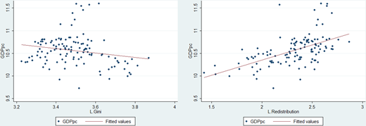
Figure 1 illustrates the findings of our econometric analysis so far. The left part shows the negative relationship between GDP per capita and inequality. The right part depicts the relationship between GDP per capita and redistribution, which appears to be positive. We will then verify the existence of this positive relationship using the appropriate econometric tools.

If we assume, as our results so far have shown, that inequality limits growth rates, then we can also assume that redistribution in favor of lower-income individuals will positively affect growth. Methodologically, we follow the same steps as in Tables 1 and 2, except that instead of the inequality variable, we use the redistribution variable. Table 3 presents the results for the augmented model.

Columns (1) and (2) are presented solely for comparison and to determine acceptable limits for the coefficients of GDPpc_{t− 1}. For the regressions in columns (3) and (4), the test results are satisfactory except for Hansen’s J test. The fully acceptable and, therefore, preferred regressions are presented in columns (5) and (6). These specific columns present stable models where the coefficient of GDPpc_{t− 1} is less than unity and within the limits set by the fixed effects and pooled OLS regressions. The Hansen and Arellano-Bond’s (AR1, AR2) tests confirm the validity of instruments and the absence of second-order serial correlation in the residuals’ differences, respectively.

Regarding the variable of interest, the coefficient of redistribution is positive under both one-step and two-step estimations, though in the latter case it lacks statistical significance. Given the small sample size, the baseline interpretation relies on the one-step estimator. Importantly, the two-step estimates remain consistent in sign and magnitude, even as statistical significance weakens. These results suggest that redistribution may positively influence growth, though the statistical significance of this effect is sensitive to the estimation method. In any case, the results do not confirm that redistribution negatively impacts growth, in line with several studies (Ostry et al., 2014; Thewissen, 2014; Cingano, 2014; OECD, 2015).

Table 4 presents the same regressions as in Table 3 but without the investment and education variables [the reduced form of equation (5)], to assess the sensitivity of redistribution’s effects on growth. Columns (5) and (6) report the regressions that satisfy the instrument validity tests and are therefore considered the preferred specifications. Both the one-step and two-step estimators confirm the positive effects of redistribution on growth, supporting robustness. The estimated effects are broadly similar between Table 3 (partial effects, net of accumulation variables) and Table 4 (total effects), indicating that redistribution operates not through the accumulation of physical and human capital but through nonaccumulation channels, potentially related to efficiency. The similarity between the reduced-form and augmented coefficients indicates that the reduced-form model is unlikely to suffer from mis-specification, such as omitted variable bias. Moreover, the loss of statistical significance in the augmented two-step specification does not reflect a substantive change in the estimated effect; rather, it is consistent with reduced precision, in line with known finite-sample properties of the two-step GMM estimator. In our data, the Okun hypothesis that redistribution generates inefficiencies is not supported; rather, the evidence suggests that inequality itself may create inefficiencies, while redistribution appears to mitigate them.

A key concern relates to the treatment of inequality as exogenous. Theoretically, this relates to the long-standing debate on growth’s effect on inequality, dating back to the Kuznets curve hypothesis. Recent contributions suggest the Kuznets curve may be empirically obsolete in modern economies (Piketty, 2014), or that “Kuznets waves” exist instead of a single curve, implying no stable, universal pattern (Milanovic, 2016). In fact, inequality is argued to be primarily shaped by institutional and policy structures, such as tax systems, labor market institutions and social transfers (Atkinson, 2015; Milanovic, 2016; Piketty, 2014).

Technically, inequality enters our specification with a one-period lag (t − 1), while growth is measured over the subsequent five-year period (t), mitigating concerns of contemporaneous reverse causality. The high persistence of inequality in our data (correlation with its lag = 0.91) has important econometric implications. It produces first differences that approach zero in magnitude, weakening instrument relevance in both equations of the System GMM estimator: lagged levels become weak predictors of first differences, while lagged differences provide little information for the level equation ^[8] (Blundell and Bond, 1998).

Finally, Difference-in-Hansen tests do not reject the additional orthogonality conditions implied by the exogeneity assumption, with p-values consistently above 0.50 across specifications. Given the temporal ordering, high persistence, weak internal instrumentation under the endogenous specification, and the absence of statistical evidence against the orthogonality conditions, we maintain the assumption of exogeneity for lagged inequality ^[9].

The analysis thus far has been based on the investigation of a linear relationship between inequality and growth. However, economic theory and previous studies suggest that the effect of inequality on growth may not be uniform across levels of inequality, implying a potential nonlinear relationship. We therefore extend the analysis to nonlinear specifications. To explore this potential nonlinearity, we introduce a quadratic term of inequality as an additional explanatory variable in regressions (5) and (6) reported in Tables 1 and 2. Collapsed instruments are used in all regressions, and the diagnostic tests yield acceptable values for Hansen’s J test as well as for the AR(1) and AR(2) tests. The results are reported in Table 5.

In regressions (1) and (2), which correspond to the augmented model, the coefficient of inequality (β1) is positive, while the coefficient on the squared term of inequality (β2) is negative, suggesting an inverted U-shaped relationship. This represents a reversed Kuznets-type pattern: inequality initially increases growth, but beyond a certain threshold further increases reduce it. This result is robust across both one-step and two-step estimators.

The reduced-form nonlinear specification, reported in columns (3) and (4), do not alter the main conclusions, as both the one-step and two-step estimators produce consistent estimates. Moreover, the coefficients on inequality from the augmented and reduced-form models, across both one- and two-step estimators, do not differ significantly, suggesting that the effect of inequality operates mainly through nonaccumulation channels ^[10].

The nonlinear relationship aligns with the notion that, at low levels of inequality, growth-enhancing incentive effects prevail, but they are gradually outweighed by the inefficiencies and distortions generated as inequality rises ^[11]. The implied turning point is calculated as (−β1)/2β2. All regressions in Table 5 yield a (log) turning point of 3.5, corresponding to a Gini coefficient of 33.1 based on the WID inequality series.

The consistency of the estimates across one-step and two-step estimators, as well as between augmented and reduced-form specifications, indicates that the nonlinear model provides a more precise characterization of the inequality–growth relationship. In contrast, the linear specification offers a valid but less refined approximation, capturing the inequality–growth nexus as a broad average negative association.

This distinction is crucial for interpreting the estimator sensitivity observed in the linear case. A literal reading of the two-step linear estimates would imply that inequality affects growth exclusively through accumulation channels and that the effect disappears once investment and education are controlled for. Conversely, the one-step linear estimates would suggest that the effect operates exclusively through nonaccumulation mechanisms, given that the coefficient remains stable when these controls are included. The nonlinear results, which remain stable across estimators and specifications, provide the appropriate benchmark for interpretation. They indicate that inequality primarily affects growth through nonaccumulation channels. They therefore suggest that the discrepancy between the linear one-step and two-step estimates does not reflect a substantive difference in the underlying economic relationship, but is more plausibly attributable to finite-sample limitations of the two-step estimator in panels with a small cross-sectional dimension.

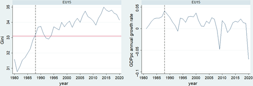
Having established the robustness and structural interpretation of the nonlinear relationship, we now examine its empirical relevance for the EU-15 economies. The estimated turning point in the inequality–growth relationship corresponds to a Gini coefficient of 33.1. Over the past two decades, the population-weighted average Gini index in the EU-15 has exceeded this threshold. A detailed picture can be obtained from Figure 2.

The left part of Figure 2 illustrates the evolution of inequality (population-weighted average Gini) for the EU-15 countries, with a reference line plotted at value 33.1. The average EU-15 Gini index exceeded this turning-point value for the first time in 1988 (dashed reference line) and definitively since the mid-1990s. This coincides with the decline in (population-weighted) average annual growth rate from 1988 onwards, as shown by the right-hand part of Figure 2. Notably, in the 1980s and 1990s, the average annual growth rate of GDP per capita in the EU-15 was 2.2% and 2%, respectively, while in the 2000s and 2010s, it did not exceed 0.7% and 0.04%, respectively. Our analysis suggests that the rising trend in inequality has contributed to the significant reduction in the average growth rate observed since 2000 in European countries.

This paper examines the effect of income inequality on economic growth in the EU-15 countries over the period 1980–2020. The conventional intuition regarding the inequality–growth nexus, rooted in mainstream approaches, builds on Arthur Okun’s (1975) notion of a trade-off between equality and efficiency, a view developed in a historical context characterized by high growth rates and declining inequality. The present study reassesses this purported trade-off under markedly different conditions, namely persistently weak growth combined with rising inequality in Europe over recent decades.

The empirical analysis is grounded in the augmented Solow framework of Mankiw et al. (1992). To address the endogeneity concerns inherent in the dynamic specification of this framework, we employ one-step and two-step System GMM estimators. A key limitation of the analysis stems from the relatively small cross-sectional dimension of the panel, an unavoidable constraint given the focus on developed and relatively homogeneous European economies. This may affect the finite-sample properties of the two-step GMM estimator and thus provides a plausible explanation for the sensitivity of some estimates. Robustness is, therefore, assessed by examining the stability and consistency of the coefficient estimates across linear and nonlinear, augmented and reduced-form versions of the MRW framework.

Four main findings emerge. First, income inequality exerts a statistically significant negative effect on economic growth. A 10-point reduction in the Gini index, approximately equivalent to the average gap between Scandinavian and Southern European countries, would increase the cumulative growth rate by about 0.8 percentage points over a five-year horizon, an economically meaningful effect given Europe’s near-zero average growth rate in recent years.

Second, income redistribution does not appear to harm growth; on the contrary, the estimates suggest that it may exert a growth-enhancing effect. Together with the negative impact of inequality, this result challenges the conventional presumption of an inherent equality–efficiency trade-off.

The third finding concerns nonlinearities in the inequality–growth relationship. Specifically, we identify an inverted U-shaped pattern consistent with a reversed Kuznets-type relationship: at relatively low levels, inequality is associated with higher growth, but beyond a threshold it becomes growth-reducing. The estimated turning point lies at approximately 33 Gini points (based on the WID inequality series), a level exceeded by the EU-15 economies in the 1990s. This threshold dynamic may help explain part of the prolonged stagnation and recurrent crises observed in Europe in recent decades.

The estimated turning point, corresponding to the late 1980s and early-to-mid 1990s in the EU-15, broadly coincides with a gradual shift toward more market-oriented policy frameworks across several European economies. This period was characterized by welfare state retrenchment, labor market liberalization and fiscal consolidation, particularly in the context of the Maastricht process and the preparation for Economic and Monetary Union. By contrast, the persistently low levels of inequality observed in Nordic economies – remaining consistently below the estimated threshold of 33 Gini points – suggest that institutional arrangements associated with the Nordic welfare state model, including universal social benefits and comparatively strong redistributive mechanisms, may be more compatible with sustained growth performance. While these associations do not establish causality, they lend institutional content to the estimated threshold and are consistent with the broader empirical finding that inequality levels beyond this range are associated with weaker growth outcomes.

Fourth, inequality appears to affect growth primarily through nonaccumulation channels. Within the neoclassical production function underlying the MRW framework, these channels correspond to the efficiency or productivity component, suggesting that higher inequality reduces the effectiveness with which human and physical capital are used. This pattern is consistent with the European experience, where other potential negative channels, such as political instability or reductions in educational attainment, do not appear to be present ^[12]. Our results suggest that at low levels of inequality, growth-enhancing incentive effects prevail; however, as inequality rises, it may foster the misallocation of resources and talent, eroding both investment productivity and the quality of human capital, thereby exerting a negative impact on growth. This mechanism helps explain why educational attainment loses statistical significance for growth despite its steady increase across countries, and underscores the importance of complementing quantitative expansion of education with improvements in quality.

This interpretation, however, is subject to an important limitation. The efficiency term in the production function cannot be directly observed or separately identified from other unobserved components in actual data. Consequently, the estimated nonaccumulation effect may also capture mechanisms outside the supply-side framework adopted here. In particular, the findings do not rule out demand-side explanations, according to which inequality may depress growth, as argued by Hein (2018), Martins (2018) and Carter (2018), among others. In this strand of the literature, reductions in consumption are frequently identified as the primary transmission channel (Kalaitzakis and Papatheodorou, 2026).

Overall, the results indicate that elevated inequality is detrimental to economic growth in the European context. Rather than confirming the equality–efficiency trade-off, the evidence suggests that beyond a certain threshold, inequality may itself generate inefficiencies, while redistribution appears capable of mitigating them. This insight is particularly relevant for Europe, where achieving higher growth rates remains a central policy priority. Our results show that redistributive policies designed to improve the allocation of resources and talent and to increase the quality of human capital without undermining productive incentives could contribute to this goal by improving the efficiency with which productive factors are used. The identification and evaluation of specific policy instruments consistent with these objectives constitute an important direction for future research.