


The purpose of the paper is to assess the fiscal sustainability of nine southern African countries that belong to the Southern African Development Community.
In this paper, the author performs a novel time-varying analysis of fiscal sustainability in southern African countries.
The authors found that in Zimbabwe and Namibia, the formal condition of solvency was not fulfilled, resulting in the explosive growth of debt during the recent slowdown. In contrast, Angola, Botswana and Malawi prove to run sustainable fiscal policies, and they were also fiscally invulnerable to the recent unfavourable economic developments in Africa. For the rest of the countries in the sample (Eswatini, Lesotho, South Africa and Zambia), the results are mixed.
In the existing literature, there is abundance of empirical evidence concerning fiscal sustainability in European and American countries. In contrast, there is strikingly little knowledge concerning this phenomenon in African countries. The authors tried to fill this gap using a novel, time-varying approach.
1. Introduction
Two recent recessions (one related to the world financial crisis and another, considerably more severe, related to the slowdown that started around 2015) raised concerns about the sustainability of fiscal policy in many African countries (Kassouri and Altıntaş, 2021). The majority of them experienced unprecedented rises in their debt-to-gross domestic product (GDP) ratio, calling into question their ability to accommodate major adverse economic shocks without diving into the payment crisis. Possible problems with fiscal sustainability are particularly growth-damaging in the context of developing countries since they may undermine the overall credibility of the ability to import capital, which may, in turn, result in abrupt capital outflows and outright economic depression.
On the other hand, the recent resurge of the fiscal theory of price level sheds new light on the unsustainable fiscal policy. According to an important strand of the literature, following the works of Davig and Leeper (2011), what was previously “unsustainable” is now sometimes viewed as an active fiscal policy that may, under some circumstances (such as the zero lower bound interest rate problem), replace monetary policy as the economy's nominal anchor.
Surprisingly, despite the growing importance of African countries in the world economy, the body of research concerning their fiscal sustainability remains surprisingly scarce. There are some works concerning a few, selected countries, including Kenya (Mutuku, 2015; Ikikii, 2017; Nganga et al., 2018; Makau et al., 2018 and Irungu et al., 2019), Algeria (Chibi et al., 2015), Nigeria (Adeosun and Adedokun, 2019), South Africa (Burger et al., 2012) and Zimbabwe (Mupunga and le Roux, 2015, 2016). There is, however, a shortage of studies for multiple (sub-Saharan) African countries. This is a surprising shortcoming since, according to Awdeh and Hamadi (2019) and Nuru and Gereziher (2021), fiscal insolvency can pose a significant threat to economic development. On the other hand, there are important studies available that use a similar methodology to what has been widely used to analyse fiscal sustainability, i.e. estimating the parameters of the fiscal reaction function to model the behaviour of fiscal authorities in African countries. Notable works include those of Agoba et al. (2019), Burger et al. (2012), Paret (2017), Lledó and Poplawski-Ribeiro (2013), Naraidoo and Raputsoane (2015), Calderón and Nguyen (2016), Konuki and Villafuerte (2016), Bouzana et al. (2018), Jalles (2017), Ouedraogo and Sourouema (2018) and Battersby and Lienert (2021). However, the main focus of those studies was on the cyclical properties of fiscal policy, such as the phenomenon of procyclicality, rather than assessing fiscal sustainability.
In this paper, we examine the fiscal solvency of nine African countries that constitute the Southern African Development Community. We argue that the available body of research is insufficient since it applies mostly the time-invariant approach to fiscal policy. As a result, in most studies, researchers present results that are averaged over some unrealistically long time. Treating fiscal solvency as something that either holds or fails to hold for many decades seems to contradict the available theory from the field of political economy (see Best et al., 2020, for recent advancements in this field). Different governments, with varying political agendas, may have fundamentally different approaches to fiscal policy. Hence, using a time-varying approach is a considerably more promising approach than averaging the parameters of fiscal reaction function over the whole sample. In this paper, we apply the state-space representation of fiscal policy and allow fiscal sustainability to be variable rather than constant characteristics of the fiscal stance. Using this approach, we show that, indeed, the overall picture is mixed: while for three countries (Angola, Botswana and Malawi) the formal condition of fiscal sustainability is met, for two other countries (Zimbabwe and Namibia), the lack of long-term solvency is coupled with recent episodes of explosive debt growth. For the rest of the sample, the picture is not clear and requires further research.
In the following section, we present a brief review of the literature, with a special focus on the fundamental assumptions underlying the testing procedures. In the third section, we present an argument in favour of treating fiscal sustainability as time-varying rather than permanent characteristics of the economy. The fourth section presents the results of the empirical assessment of fiscal solvency for the group of nine southern African countries. The last section concludes.
2. Fiscal sustainability–review of the literature
Fiscal sustainability can be defined as the ability of the public sector to fulfil its financial obligations in a timely manner (Quintos, 1995; Bohn, 2005). This means that the public sector satisfies the intertemporal budget constraint, according to which the current value of the expected primary surpluses equals the present public debt. This condition (as a percentage of GDP) can be expressed as:
where bt, ht and gt denote the ratio of debt, revenues and primary expenditures, respectively, to GDP, g is the long-run GDP growth rate, and r is the long-run interest rate [1]. (1) is equivalent to the current value of the public debt being convergent to 0:
which is the transversality condition of the intertemporal decision problem of the public sector. A number of methods have been used in the literature to test whether this transversality condition is met.
Historically, Hamilton and Flavin (1986) were the first to show that the stationarity of public debt can be viewed as a sustainability condition, since the exponential decay term algebraically dominates the mean-reverting debt term in (2). This approach was then followed by several authors, including Kremers (1989), Trehan and Walsh (1991), Hakkio and Rush (1991), Corsetti and Roubini (1991), Buiter and Patel (1992), MacDonald (1992), Artis and Marcelino (1998), De Castro and De Cos (2002), and Bravo and Silvestre (2002). Besides the standard augmented Dickey–Fuller (ADF) test, a number of different tests are commonly used to examine the stationarity of deficit and debt, including the Phillips–Perron test (1988), the Kwiatkowski et al. test (1992), the Elliott, Rothenberg and Stock Point Optimal test (1996), as well as the Ng and Perron test (2001).
Despite its popularity, this approach suffers from important shortcomings. Bohn (2005) presented formal proof that the exponential decay dominates the debt term if the latter is of any finite order. Hence, testing for debt stationarity presents only a sufficient, but not a necessary condition for fiscal solvency. Another problem is more of an empirical nature: it is widely recognised that stationarity tests suffer from low power in short samples (see, e.g. DeJong et al., 1992). This issue is particularly serious in the context of fiscal data since the recorded history of fiscal variables rarely covers more than 50 years. Also, a simple univariate approach tells us little about the underlying mechanisms of achieving fiscal sustainability. As pointed out by Alesina et al. (1998), there are important differences in the effectiveness of fiscal consolidations that depend on their reliance on the revenue or expenditure sides of the budget.
In order to at least partially address these problems, some authors used a cointegration analysis as a test of fiscal sustainability. MacDonald and Speight (1990) and MacDonald (1992) were the first to analyse the cointegration relationship between debt and deficit. This approach was also followed by Artis and Marcelino (1998). The presence of such a long-run cointegration relationship was deemed proof of fiscal solvency. Hakkio and Rush (1991) tested cointegration between revenues and total expenditures to check fiscal sustainability. This approach was widely followed by, among others, Tanner and Liu (1994), Haug (1995), Quintos (1995), Afonso (2005) and Marinheiro (2006). Several authors (including Ahmed and Rogers, 1995 and Claeys, 2007) extended this approach and tested for the presence of a cointegrating relationship between revenues, primary expenditures and interest payments.
To overcome the problem of the low power of the tests, many authors used panel models, since they make it possible to work on many more data points. Claeys (2007) was among the first to apply panel stationarity and cointegration tests as a tool to assess fiscal sustainability in the European Union (EU). Adedeji and Thornton (2010) performed an analysis for a panel of Asian countries, Campo-Robledo and Melo-Velandia (2015) for Latin America, while Mahdavi and Westerlund (2011) performed a similar assessment on a regional level for a panel of American states. While these methods truly allow the use of larger samples, thus potentially increasing the power of the tests, they raise the issue of panel homogeneity. Most methods test a null of integration against the alternative of stationarity of at least one entity in the panel. Thus, a test that rejects the null hypothesis does not necessarily mean sustainability in all countries–instead, it means that fiscal policy is sustainable in at least one country.
An important weakness that panel analyses of fiscal sustainability commonly suffer from is that clustering different countries in one panel often lacks firm theoretical foundations. The authors of the cited papers rarely explain why they chose to treat such diverse economic agents, such as the governments of different countries, as if they behaved (almost) the same way and could thus be modelled using a single behavioural equation.
In order to address the problem of the non-conclusiveness of fiscal sustainability tests, Henning Bohn, in a series of papers (1998, 2007, 2008), proposed an approach that relies on estimating the parameter of the so-called fiscal reaction function (FRF). The FRF is a behavioural equation whose objective is to model the fiscal surplus (or, alternatively, debt growth) as a function of different independent variables, suggested by the theory of political economy and public choice. It can be viewed as a fiscal analogue to the monetary Taylor rule. Typically, it takes the form:
where s is a measure of the surplus (or deficit) of either central or general government, b is debt, and x is a vector of other important determinants of fiscal stance, such as inflation and one-off revenues. In order to use the FRF as a tool to assess fiscal sustainability, Bohn (1998) proposed using primary surplus as the dependent variable. He presented formal proof that the estimated sign of parameter is then decisive for fiscal sustainability: for any , public finances are sustainable. Moreover, if the relationship between debt and surplus is linear, this condition also becomes a necessary one (in contrast to the integration approach, where it is only sufficient), since if this parameter is zero or positive, this process generates an explosive debt series, with a rate that is sufficient to violate (2). The condition of linearity is important in this context since, for a non-linear relationship, sustainability may hold even if this condition is not met. Bohn (2007) points to a case when initially but turns positive when debt exceeds some finite level. Such behaviour of fiscal authorities is consistent with the condition of sustainability, even though the locally positive relationship between surplus and debt may not be observed.
A large group of researchers soon followed this approach. For example, it was used by Jayawickrama and Abeysinghe (2007) to test the sustainability of US public finances, by Ballabriga and Martinez-Mongay (2005) to analyse EU public finances, by Claeys (2006), Giannitsarou and Scott (2006), and Mendoza and Ostry (2008) to test sustainability for a panel of OECD countries, by Greiner et al. (2007) to test fiscal stability in Germany, and by Haber and Neck (2006) to analyse Austrian public finances. Still, this approach suffers from at least two weaknesses. First, by treating the sample as a whole, it may fail to detect short-lived episodes of fiscal insolvency. We argue in this paper that this is a fundamental flaw that undermines the economic sense of using this method. Second, while it is certainly a step in the right direction, this method still fails to provide a decisive test for fiscal sustainability, i.e. it is possible that parameter ρ is not only non-constant over time but that it takes different values depending on the level of debt. Bohn (2007) points to a case where this parameter is zero for lower levels of debt while taking positive values for higher levels. In this case, sustainability would be ensured even when a quantitative relationship between debt and surplus (i.e. ) would be non-detectable in “normal” times of relatively low levels of public debt.
3. Empirical methods
Although several of the cited scholars chose to allow for the time-varying behaviour of the fiscal authorities, a dominant strand of the literature treats fiscal sustainability as a permanent characteristic of the economy (Bystrov and Mackiewicz, 2020). Fiscal policy is tested to be either sustainable or unsustainable over the whole sample, which can be anywhere between a few decades to over two hundred years (as in the case of two countries with the longest recorded fiscal history, i.e. the US and the UK). However, this approach suffers from an important inconsistency. We argue that potential fiscal unsustainability over such long periods would be inconsistent with the long-run rationality of fiscal authorities, voters and lenders.
For a moment, consider the unrealistic scenario of a long-run fiscal policy violating the solvency condition (3). In line with the reasoning presented by Bohn (2007), it is not sufficient that debt is tested to be integrated of order one or higher. For public finances to be unsustainable, the debt-to-GDP ratio would need to follow an explosive path, at an average growth rate greater or equal to . If it grows with a rate of exactly , this is a special case when the government does not pay any interest, hence keeping the zero-primary balance. Any negative primary balance results in a growth rate of debt that exceeds .
However, running such a policy, in the long run, is not solely the decision of a government. In a democracy, it needs the support of voters, who should be nearly indifferent to fiscal problems. This means that voters should systematically fail to recognise the risk of a fiscal crisis (also in the long run). Moreover, to provide financing for such a policy, lenders should also be myopic enough to ignore the risk of eventual default. Both assumptions are hard to reconcile with the rational behaviour of voters and investors, particularly in the long run.
Modelling fiscal policy as a time-invariant phenomenon encounters yet another problem, rooted in political economy. A number of studies confirm a strong connection between election outcomes and fiscal policy (for example, see Tiganas and Peptine, 2012 for a thorough review of the literature on the political business cycle). In the light of this literature, it is a far-fetched simplification to assume that fiscal policy is invariant to election outcomes. Another strand of the literature shows that fiscal institutions have a strong impact on a fiscal programme (see von Hagen, 1992; Alesina et al., 1996; Wyplosz, 2005). While fiscal institutions change slowly and infrequently, they do change, and it is implausible to assume that this process has no impact on fiscal sustainability. Hence, fiscal sustainability is, in general, not a characteristic that would remain constant over decades. If this is the case, an analysis of long-run fiscal sustainability based on a time-invariant model involves unjustified averaging over different fiscal regimes. Some of these regimes are likely to be sustainable, while others can truly violate the intertemporal solvency condition.
This calls for a set of methods that would allow sustainability to be a transitory rather than a permanent characteristic of the behaviour of fiscal authorities. Indeed, the time-varying models of fiscal policy have been applied in a few studies so far. Cipollini (2001) used a model with smooth transition error correction, while Arestis et al. (2004) applied threshold regression to assess fiscal sustainability in the US. A fiscal reaction function with Markov switching was estimated in a series of papers by Leeper et al. (2010), Davig and Leeper (2011), and Bi and Leeper (2013). Using this approach, they were able to distinguish between sustainable and unsustainable fiscal policies in US history. Another way to allow for time-varying parameters was to apply models with one or multiple structural breaks. Afonso (2005) and Afonso and Jalles (2012) combined this approach with panel models in order to assess fiscal sustainability in EU countries [2].
However, so far, these methods have been applied almost purely to a few highly developed countries with long available recorded fiscal history, such as the United States, United Kingdom or Sweden (Bystrov and Mackiewicz, 2020). In this paper, we extend their use to a group of southern African countries to analyse if there have been any serious episodes of unsustainability in recent history and, in particular, how they responded to the two most recent economic slowdowns that might result in severe fiscal problems.
One of the widely applied methods to tackle the task of estimating models with time-varying parameters is the use of Kalman filters. This method, first developed by Swerling (1959) and Kalman (1960), has been widely applied in fields such as navigation and global positioning (Kaplan and Hegarty, 2005; Strang and Borre, 1997), robotics (Roumeliotis and Bekey, 2000), fault detection (Isermann, 1984) and computer vision (Ridder et al., 1995). Harvey (1990) showed its applications in the area of econometrics and time-series analysis. It makes it possible to model complex time series with unprecedented flexibility, including multiple latent random variables and time-varying regression parameters. Its application requires the underlying economic model to be presented in the so-called state-space form (Harvey et al., 2005).
where (4) is the so-called observation equation with the vector of observable variables and (5) is the state equation that describes the evolution of a vector of latent variables . The task to assess fiscal sustainability in a manner that would allow the parameter ρ to vary over time, for each country i independently, requires the following set of equations to be specified:
where , , and denotes the output gap.
Both fiscal surplus and debt are expressed as a per cent of GDP, while the output gap is expressed as a per cent of potential GDP. In order to ensure the stock-flow relationship that is required for (2) to be a condition for sustainability, we used the definition of .
4. Data and empirical results
The data on public debt refer to central government debt expressed as per cent of GDP and come from the Global Debt database provided by the International Monetary Fund (Mbaye et al., 2018). The data on GDP come from the Penn World Table 9.1 (Feenstra et al., 2015) and were used to calculate the output gap. Following Seetharam and Britten (2015), among others, we calculated the output gap using the Hodrick–Prescott filter with the smoothing parameter set in accordance with the Ravn-Uhlig rule for annual data [3]. Due to its short recorded history of 17 years of fiscal policy, we decided to omit Mozambique (which also formally belongs to the Southern African Development Community), which left us with a group of nine countries.
Table 1 presents the basic summary statistics of our data. The analysed countries differ considerably both in terms of the level of public debt and their variability. The ratio of public debt to GDP turned out to be a non-stationary variable, which is consistent with the smoothing behaviour of fiscal authorities (Barro, 1979). On the other hand, the output gap is, as expected, a stationary variable with zero mean and standard deviation that equals several percentage points.
Summary statistics
| Country | N | Debt to GDP, % | Output gap, % | ||||
|---|---|---|---|---|---|---|---|
| Mean | S.D. | ADF | Mean | S.D. | ADF | ||
| Angola | 23 | 0.76 | 0.54 | −2.77* | 0.00 | 0.07 | −2.74* |
| Botswana | 46 | 0.19 | 0.11 | −2.49 | 0.00 | 0.05 | −3.69*** |
| Eswatini | 47 | 0.16 | 0.04 | −1.66 | 0.00 | 0.06 | −4.61*** |
| Lesotho | 47 | 0.52 | 0.30 | −1.48 | 0.00 | 0.07 | −3.61*** |
| Malawi | 47 | 0.56 | 0.29 | −2.26 | 0.00 | 0.04 | −4.79*** |
| Mozambique | 19 | 0.71 | 0.32 | −0.83 | 0.00 | 0.04 | −3.80*** |
| Namibia | 29 | 0.23 | 0.08 | −2.17 | 0.00 | 0.03 | −2.88** |
| South Africa | 47 | 0.37 | 0.07 | −0.40 | 0.00 | 0.02 | −3.58** |
| Zambia | 47 | 0.39 | 0.56 | −2.44 | 0.00 | 0.03 | −4.02*** |
| Zimbabwe | 47 | 0.38 | 0.16 | −0.18 | 0.00 | 0.10 | −2.56 |
Note(s): Levels of statistical significance: *p < 0.1, **p < 0.05, ***p < 0.01
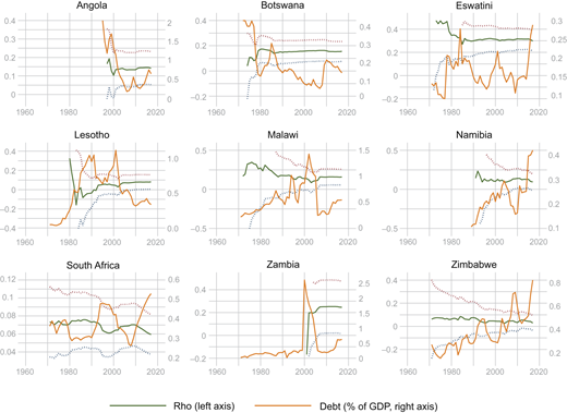
Table 2 presents the results of the estimation of equations (6) and (7) performed using the Kalman filter. Since the values of , which is a parameter of interest in our study, change every year, we decided to present them graphically (Figure 1). In addition to the values of estimated , it also shows the public debt-to-GDP ratio. Due to the existing stock-flow relationship between left- and right-hand variables, the calculated t statistic does not have the student distribution; hence, the standard confidence interval would be biased–too narrow, due to underestimated variance. Thus, in order to calculate the 5% confidence intervals for that are presented in Figure 2, we decided to use the critical values of the distribution.
Estimated coefficients
| Country | ||||
|---|---|---|---|---|
| Angola | −0.058 | 0.895 | −3.320 | 0.017 |
| Botswana | −0.022 | 0.165 | −0.282 | 0.001 |
| Eswatini | −0.048 | −0.069 | 0.052 | 0.011 |
| Lesotho | −0.187 | −2.689 | −3.493 | 0.026 |
| Malawi | −0.093 | 1.475 | −1.741 | 0.021 |
| Mozambique | −0.031 | −0.225 | 0.071 | 0.002 |
| Namibia | −0.048 | 0.106 | −0.102 | 0.001 |
| South Africa | −0.023 | 0.616 | −0.491 | 0.001 |
| Zambia | −0.106 | 1.027 | −0.463 | 0.129 |
| Zimbabwe | −0.017 | 0.346 | −0.032 | 0.003 |
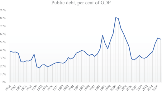
Public debt in the Southern African development community, % of GDP, unweighted average
Public debt in the Southern African development community, % of GDP, unweighted average
There are several major findings that can be observed from our estimation results. First, with some exceptions, the estimated values of parameter remained relatively stable over the sample. This is particularly surprising since recent times have been particularly shaky in terms of fiscal and economic conditions, resulting in the growth of debt in many African countries. Among the analysed countries, only South Africa has recently presented clear signs of diminishing fiscal sustainability. In the case of Namibia and Zimbabwe, similar tendencies are also visible, although they are much shorter-lived and less pronounced, at least in relative terms.
Of the analysed countries, Zimbabwe and Namibia can be classified as having outright problems with fiscal sustainability. In recent years, in both cases, the value 0 lies within the 5% confidence interval. This means that for conventional significance levels, there is a chance that may be zero, which means a possible violation of the transversality condition (2). The indicator of fiscal sustainability has also had a subtle downward trend in the last few years, creating bad prospects for the future. In these two countries, the level of public debt has also reached unprecedented levels in the last few years, which, together with the estimated values of , raises clear concerns about fiscal sustainability in these countries.
Lesotho, despite not formally fulfilling the sustainability condition, turned out to be a borderline case. While was not above 0 in a statistically significant way during most of the sample, the recent trends are certainly promising. A subtle yet noticeable positive trend in could be observed, rendering the lower bound of the confidence interval slightly above 0 in the last few years of the sample. The country managed not only to cut its debt considerably after 2000 but also to sustain this downward trend after 2010, during the years of the crisis. Hence, it seems justified to consider fiscal policy in Lesotho as currently sustainable, although the definite classification is yet to be seen.
For the other six countries in our sample–Angola, Botswana, Eswatini, Malawi, South Africa and Zambia–the estimation results are considerably more promising. In all cases, zero lies clearly outside the 5% confidence interval, which is a strong case for the sustainability of fiscal policies in these countries. However, this picture is not complete without supplementing it with the dynamics of public debt. Among this group of countries, Angola, Botswana and Malawi have managed to curb the growth of public debt-to-GDP ratio in recent years, despite the unfavourable conditions for fiscal policy in Africa in general. In contrast, Eswatini, South Africa and Zambia are countries where an explosive growth of debt can be observed within the same period. Hence, in this last group of countries, the results are mixed. Our interpretation is that while these countries historically have been characterised by a sustainable fiscal policy (as indicated by estimation results based on the full sample), their most recent fiscal performance is questionable. It is yet to be seen if these unfavourable changes remain on-off or turn into trends that can, over time, also negatively affect the degree to which the formal condition of sustainability is fulfilled.
5. Conclusions
Our analysis shows that the group of southern African countries–members of the Southern African Development Community–is surprisingly heterogeneous in terms of fiscal policy sustainability. Our results show that while fiscal regimes fluctuated in the past, within the last ten years, the picture in each country remains stable.
For two countries, the results are consistently negative: in both Namibia and Zimbabwe, we observed no reaction of fiscal surplus to the level of public debt that would ensure sustainability. As a result, their ratio of public debt to GDP has skyrocketed in recent years, and it may require serious fiscal efforts before it returns to more acceptable levels. On the other end of the sustainability continuum are three countries with reputable fiscal histories: Angola, Botswana and Malawi. In these countries, the fiscal policy proves to react to the changing economic environment in a way that prevents the level of debt from exploding, thus ensuring that the fiscal solvency holds. During the recent economic slowdown, they managed to curb their debt growth or even, in the case of Botswana, reduce the level substantially. The other four countries present a mixed picture. Lesotho proves to have an excellent recent history of debt reduction, while its fiscal reaction parameter reached a sustainable level only in the last few years. The opposite is true of Eswatini, South Africa and Zambia. In these countries, the formal condition of fiscal sustainability is met, yet it has been coupled with the rapid growth of public debt in the most recent period. Hence, the ability of the fiscal authorities in these countries to restore moderate levels of public debt is open to question.
In this study, we used the theoretical approach that views fiscal sustainability as a variable rather than a permanent property of fiscal policy. While this approach is not entirely new, it has been largely neglected in most previous studies on fiscal sustainability. Treating fiscal solvency as a constant property of fiscal policy seems to find little support in the available studies on political economy. Successive governments may (and often do) have different policy objectives and, therefore, different approaches to maintaining a good fiscal stance. As a result, fiscal sustainability, although itself a long-term feature of fiscal policy, may vary from year to year. Therefore, a flexible approach to measuring it seems to be more sound and better rooted in available political and economic theory than the bulk of the available research.
5.1 Limitations of the study
In this paper, we have tried to provide insight into the fiscal sustainability of African countries. However, our analysis has certain limitations that come from data availability and the choice of method. Because of the lack of data regarding spending on interest on public debt during the whole period, we were unable to use the primary surplus as the left-hand side of the fiscal reaction function, as suggested by Bohn (2007). Instead, we decided to use debt growth, which makes our sustainability test a sufficient rather than a necessary condition for fiscal solvency. However, it should be noted that, since we performed the estimation for variables expressed in per cent of GDP terms, the difference is small, since it amounts to , where g denotes the nominal GDP growth rate and r is the nominal interest rate. In a dynamically efficient economy, this difference is positive, yet small on average. It should be expected that performing the same test using the primary surplus (rather than a decrease of debt) could bring less stringent results, i.e. more countries could be viewed as fiscally sustainable. In particular, this refers to the group of four countries for which the results of our tests were not clear.
Also, in our study, we used a univariate approach; thus, we did not make use of possibly valuable information concerning the composition of fiscal adjustments. This was due to the fact that the available time series on public debt was considerably longer than that for fiscal surplus, revenues and expenditures. However, should such data become available, performing a detailed analysis of revenue and expenditure roots of fiscal developments is a promising avenue for further research.
Notes
It is worth noting that this solvency condition makes sense only in a dynamically efficient economy, where .
Paparas et al. (2015) provide a more comprehensive review of the recent studies.
For comparison, we also performed estimations using the Christiano–Fitzgerald filter when calculating the output gap. The results were very similar and hence have not been reported here.

