Data envelopment analysis and data mining to efficiency estimation and evaluation

Sustainability is one of the concepts which has been associated with bank performance; therefore, assessing and predicting bank performance have become vital for managers when examining the suitability of their managerial decisions. Additionally, studying bank performance greatly facilitates measuring the success of decisions made by a bank as compared to those of its counterpart during the same period. Furthermore, it allows one to learn how to make better financial decisions that allocate financial resources in a more efficient manner. There is substantial body of published academic research that discusses different methods of evaluating bank performance; Berger and Humphrey (1997) grouped them into two main approaches, namely, parametric and nonparametric. The most popular parametric method is known as the stochastic frontier approach (SFA), whereas the most popular nonparametric method is data envelopment analysis (DEA). Although using these methods could help researchers determine performance level, they are not sufficient to explain inefficiency or predict performance. Therefore, several studies, like that of Fethi and Pasiouras (2010), proposed a combination of measuring and explaining bank performance using DEA or SFA in the first stage to measure performance and regression models as a second stage to explain it. Casu and Molyneux (2003); Ariff and Can (2008) and San et al. (2011) used Tobit regression in particular to explain bank performance. Other researchers used different regression models to explain bank performance; Anouze (2010); Emrouznejad and Anouze (2010) and Bou-Hamad et al. (2017) used boosted generalized linear model, and Seol et al. (2007) used decision trees, whereas Azadeh et al. (2011) used the artificial neural networks (ANNs). On the other hand, Sun and Li (2008) and Wu and Hsu (2019) used decision tree techniques to introduce a multiple criteria decision-making method to determine suitable warning mechanisms of corporate financial failure or distress. Meanwhile, Lai et al. (2011) used DEA to develop an intellectual benchmarking knowledge-based system for benchmarking, performance evaluation and process improvement.

However, no comparison of methods used in second DEA stage has been made, and most of these studies aimed only to explain the factors affecting efficiency rather than predicting future efficiency of banks. Predicting bank performance is extremely important: bad performance may lead to bankruptcy, which negatively influences the economy of a country. Thus, conceiving a powerful predictive model for bank performance would be useful in avoiding or at least limiting such consequences. Therefore, this study proposes a comprehensive performance evaluation framework based on managerial, financial and macroeconomic indicators to predict bank performance. More specifically, seven predictive techniques, namely, classification and regression trees (CART), conditional inference trees (CIT), random forest based on CART (RF-CART), random forest based on CIT (RF-CIT), bagging, ANNs and logistic regression (LR) are assessed when applied to second-stage DEA. This framework is applied to a data set of 151 banks from Middle East and North Africa (MENA) countries observed over a period of three years (2008-2010); hence, the data set contains 453 observations with 15 environmental variables (predictors). For predictive comparison among the used data mining methods, we used the overall accuracy, sensitivity, specificity and the areas under the ROC curve (AUC).

The following sections are organized as follows: Section 2 reviews the related literature and Section 3 describes DEA and data mining methods used. Section 4 describes the MENA banks data set. The experimental set up and model performance measures used in our comparison are described in Section 5. Finally, we present and discuss our results in Section 6, and we conclude in Section 7.

Several authors investigated the influence of environmental conditions on bank performance. Linear regression analysis is one of the most popular statistical techniques used in performance measurement. However, in practice, researchers have used regression analysis for both prediction and explanation of a firms’ performance level (Azen and Budescu, 2003; Courville and Thompson, 2001; Johnson and LeBreton, 2004; Pedhazur, 1997). The linear regression result is not particularly well suited, as it is a common nature of the environmental variables to be correlated (Grömping, 2007).

Hence, other approaches to investigating the impact of environmental variables on performance were proposed. Ray (1988) proposed using a two-stage method; the first stage consisted of measuring bank efficiency using DEA, while in the second stage, the obtained DEA efficiency score of each bank is regressed against selected environmental variables using SFA. Later on, Ray (1991) proposed using a regression analysis in which the environmental variables are regressed on efficiency scores rather than the SFA. The second stage method (two-stage analysis), which is the most common method used among researchers (Ariff and Can, 2008; Casu and Molyneux, 2003; San et al., 2011), is seen as a solution for the impact of variables that are not included in the initial DEA model. In addition, Fried et al. (2002) recommended using three-stage analysis; the first stage comprised computing the efficiency score using DEA model. Then the total slack of the input and output constraints, [i.e. x – Xλ ≥ 0 and Yλ – y ≥ 0] which is the source of inefficiency, is considered to have three effects: managerial inefficiencies, environmental influences and measurement error (statistical noise). In the third stage, SFA is used to estimate values for these components. Estelle et al. (2010) proposed a different three-stage framework, and their results show that the one-stage model is unable to decompose the efficiency and environment effects, which point out the weak performance of the one-stage model.

Alternative powerful methods such as CART (Anouze, 2010; Emrouznejad and Anouze, 2010); Seol et al., 2007) and ANNs (Azadeh et al., 2011; Toloo et al., 2015; Hanafizadeh, et al., 2014) were considered to complement the classic statistical genetic methods.

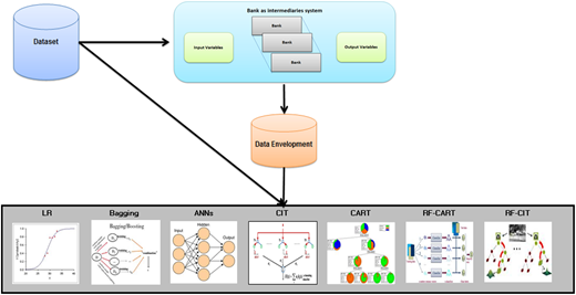
The framework starts with DEA computation of the performance of each bank, and the efficiency scores obtained are grouped accordingly into efficient banks (efficiency score of 1, target = 1) and inefficient banks (efficiency score less than one, target = 0). This classified efficiency score is used as a target, while the environmental (exploratory) variables are used as inputs of data mining techniques. Figure 1 depicts our proposed framework.

In the following paragraphs, we briefly describe the DEA and the seven prediction techniques used in our study.

DEA is a non-parametric method developed by Charnes et al. (1978) to measure the performance of set decision-making units (DMUs) (Emrouznejad et al., 2008 and Emrouznejad and De Witte, 2010). The initial DEA models consider constant return to scale (CRS) which ignores the fact that different DMUs (banks) could be operating at different scales. To overcome this drawback, Banker et al. (1984) introduced variable returns to scale (VRS) model, which ensures that each bank is only benchmarked against banks of similar size. To introduce DEA-VRS model, assume there are n banks (aj = 1,…,n) using m inputs (x_ij i = 1,…,m) and producing s outputs (y_rj, j = 1,…,s). DEA measures the technical efficiency of bank j₀ compared to n peer group of banks input and output. DEA formulation in Models (1a) assesses bank_j0 under VRS, where the efficiency of bank_j0 is the optimal value of θ. This model is described as input oriented. Similarly, an output-oriented DEA is defined in Model (1b) where the efficiency of bank_j0 is the optimal value of 1/∅ (Thanassoulis, 2001).

Model 1a. Standard input-oriented DEA-VRS

subject to

Model 1b. Standard output-oriented DEA-VRS

subject to

To reach to CRS-DEA, one can remove $∑j=1nλj=1$ constraint from the above models.

However, DEA alone determines only the efficiency scores of each bank and does not account for the factors related to inefficiency; neither can it predict the performance of each bank (Emrouznejad and Anouze, 2010) nor account for flexible measures variables (Amirteimoori and Emrouznejad, 2011; Amirteimoori and Yan, 2014) and the uncertain nature of the future (Amirteimoori et al., 2013).

LR is a generalization of linear regression (Hosmer and Lemeshow, 2000) used for predicting a dichotomous dependent variable (efficient, inefficient) or multi-class-dependent variables. LR assumes that the response variable is linear in the coefficients of the predictor variables. In this study, LR analysis is performed with financial and economic data related to bank performance to assess the independent effect of each factor. The specific form of a logistic model is as follows:

where x₁,…,x_m are m explanatory variables. LR produces a simple probabilistic formula of classification, and this is its main advantage. However, the weakness is that LR cannot deal with the problems of non-linear and interactive effects of explanatory variables (Yeh and Lien, 2009).

A classification and regression tree is a non-linear discrimination method that uses a set of independent variables to split a sample into progressively smaller subgroups. Tree-based methods have appeared with Morgan and Sonquist (1963). However, they gained their popularity through the major theoretical and practical contribution of Breiman et al. (1984). It was initially introduced as an alternative to parametric methods in discriminant and regression analysis and has been extended more recently to censored survival analysis (LeBlanc and Crowley, 1992; Bou-Hamad et al., 2009; Bou-Hamad et al., 2011). CART uses a recursive algorithm to split the data into classes (or nodes) based on logical if-then conditions on the explanatory variables. The splitting criteria of classification trees aim to find the best splitter explanatory variable portioning the parent node into two more homogenous children nodes. The algorithm starts with the root node (initial data set) and so on until growing a large tree. For classification trees, the goodness of the split is measured by the impurity function defined as follows:

where s is the candidate split of a variable (v, t) the parent node, i(t) the impurity of the node t p_L and p_R the proportions of objects going to the left (t_L) or right (t_R) child nodes, respectively, and i(t_L) and i(t_R) their impurities. Several impurity measures have been proposed, and the most popular ones are the deviance and the Gini index. The impurity measure is defined as $i(t)=−∑j=1cpj(t)ln⁡(pj(t))$ for the deviance and $i(t)=1−∑j=1c(pj(t))2$ for the Gini index, where p_j(t) is the proportion of objects in node (t) that belong to the j^th class of the (C) classes present in the data set.

The growth of the tree can be continued until no further splits are possible. However, fully grown trees tend to over-fit the data, which is why a stopping criterion is needed. Breiman et al. (1984), proposed a pruning algorithm in which a large tree is grown then pruned back to produce a set of nested trees from which the final tree will be selected.

The main advantage of classification trees is the simplicity of interpreting their results. Another advantage is that classification trees do not require implicit assumptions as in the case of parametric models. Despite their advantages, decision trees suffer from instability (Breiman et al., 1984), where a small change in the training data may have a major impact on the predictive ability of the tree.

Unlike CART where its splitting criterion is based on impurity reduction, the CIT recently proposed by Hothorn et al. (2006b) use a splitting criterion based on multiplicity-adjusted conditional tests (Hothorn et al., 2006a). For any node, the splitting procedure consists of conducting a global permutation test of no association between any predictor variable and the response within the node. If the global hypothesis of no association is not rejected, the node is not split and is considered a terminal node. Otherwise, for each predictor, an individual null hypothesis of no association with the response will be conducted. The predictor with the lowest p-value is selected for splitting. In CIT, pruning is not required as the trees stop growing when the split is not statistically significant.

A single tree is unstable in the sense that small perturbations in its training set may result in changes in its predictions (Breiman, 1996). Using ensemble methods such as bagging and random forests often produces better performances than using a single tree. Bagging is a bootstrap ensemble method introduced by Breiman (1996). It can be used with many classification methods and regression methods to reduce the variance associated with prediction and therefore improve the prediction process (Sutton, 2005). Hence, it consists of averaging the fitted values of the response variable of many trees built with bootstrapped samples from the original data. Basically, it trains each classifier on a randomly drawn training set; each classifier’s training set consists of same number of banks randomly drawn from the original training set, with an equal probability of drawing any given bank. These samples are drawn with replacement so that some banks may be selected multiple times, while others may not be selected at all. As a result, each classifier could return a higher test set error than a classifier using all of the data (Kim, 2006). However; when these classifiers are combined (typically by voting), the resulting ensemble produces a lower error on the test set than a single classifier. Bagging has been found to be the simplest algorithm that helps in reducing variance and improving unstable classifiers in accuracy (Breiman, 1996). It also enhances accuracy when random features are used and can help avoid overfitting. However, the disadvantage of bagging is that bagged trees are not as easily interpretable as a single tree (Zhu, 2010).

Breiman (2001) originally introduced the random forest as an ensemble of CART trees (RF-CART). This method gives a prediction based on the majority voting (the case of classification) or averaging (the case of regression) predictions made by each tree in the ensemble using some input data (Antipov and Pokryshevskaya, 2012). In this sense, it is similar to the bagging technique, and it combines many individual decision trees to provide a final prediction. However, the key difference between them is that bagging uses an exhaustive search of all the explanatory variables to find the best split, while RF uses a randomly selected set of explanatory variables at this step. Recently, Strobl et al. (2007) developed a random forest based on conditional inference trees (RF-CIT). The general method of both RF-CART and RF-CIT can be outlined as follows:

• Draw B bootstrap samples from the data,

• Grow a tree for each bootstrap sample. At each node, select at random k out of m covariates on which to base the decision at that node.

• Each tree is fully grown and not pruned. The splitting is stopped when a minimum node size is reached.

RF suffers from the same problem of interpretation as bagging does. However, several techniques have been developed for RF to allow for interpretation. The most useful one is the variable importance; the common and frequently used variable importance measure is the permutation-based mean decrease in accuracy (Breiman, 2001). This measure allows researchers to identify a set of important variables that can potentially affect the dependent variable.

ANNs are one of the most commonly used data mining models for prediction. An ANN is inspired by the structure of biological neural networks where neurons are interconnected and learn from experience. Neural networks are composed of nodes (neurons) arranged in layers that are fully connected to the preceding layer via a system of weights. Numerous different neural network architectures have been studied. However, the most successful applications of neural networks have been multilayer feed forward networks. These are networks in which there is an input layer, one or more hidden layers and an output layer. The input layer is where the input features are fed and forwarded to the hidden layer, which is again forwarded to the output layer.

The output of a hidden layer node is computed in the following manner. First, a weighted sum of inputs is computed and then a transfer function is applied to this sum. More specifically, for a set of input values, x₁,x₂,...,x_m, the output of node j is computed by taking the weighted sum $θj+∑i=1mwijxi$⁠, where θ_j,w_1j,...,w_mj are weights that are initially set randomly and adjusted as the network learns. The next step is to apply a transfer function g to this sum. A transfer function is a monotone function. The most popular transfer function is the logistic function g(s) = 1/(1 + e^−s). Finally, the output layer obtains input values from the hidden layer and the same transfer function is applied to create the output (Shmueli et al., 2010, pp. 222-229).

The common algorithm used to estimate and update the weights is the back-propagation (Rumelhart et al., 1986). However, this algorithm suffers from a low learning speed (Castillo et al., 2006). Many alternatives have been proposed to increase the learning speed. One of them is a general quasi-Newton optimization procedure, the Broyden-Fletcher-Goldfarb-Shanno algorithm that is used in this paper.

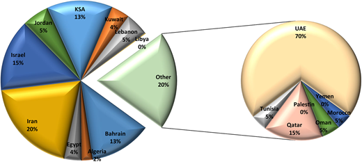
The proposed methodology is applied to a sample of banks operating in MENA countries over the period of 2008-2010. The period after 2011 was witness an Arabic Spring movement that impacted the performance of banking sector in these countries; therefore, these years were excluded to avoid any up-normal variation in bank performance. The total number of banks operating in MENA countries over the selected period was 535 banks, however due to data availability only 151 banks (Appendix A) are included. The sample includes data from Lebanon (27 banks); Egypt (21); United Arab Emirates (18); Bahrain; Israel and Jordan (13 banks each); Saudi Arabia (11); Oman (7); Qatar and Tunisia, (6 banks each); Iran and Kuwait (5 banks each); Algeria (2) and Libya; Morocco; Yemen and Palestine (1 bank each). Figure 2 illustrates their share of assets.

Although our sample consists of banks from various countries with differing accounting regulations, we believe the accounting data are comparable across the whole sample, as the financial statements data optioned from Bankscope are reported in a unified global format.

In general, different set of input and output variables were used in various studies. A debatable concern usually occurs when it comes to classifying a variable as either an input or an output due to varying definitions. There are three main approaches used as a base to select and classify the input and output variables: production, intermediate and value-added approach. Other researchers used a mix approaches. The first approach popular in branches efficiency studies was that bank is treated as a vendor who use labor, capital and equipment to produce various number of deposits and loans transactions. The second approach treats banks as intermediaries between savers and investors, hence variables such as labor or labor cost and deposits and assets were frequently used as inputs and variables like loans, securities and investments were frequently used as outputs.

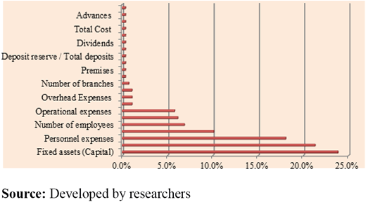
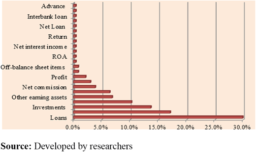
In this study, for the purpose of measuring bank performance and comparing different data mining techniques in predicting the performance, an in-depth analysis of previously published literature was conducted to select the most popular input and output variables. A total of 204 published were reviewed and analyzed in term of used inputs, output and environmental variables. In term of DEA input and output variables, most of the reviewed literature relied on bank’s balance sheet. Figure 3 illustrates the most used input variables, whereas Figure 4 illustrates the most used DEA output variables and Table II illustrates the most used environmental variables and the used statistical test to study the impact of the environmental variables on bank performance.

Figure 3 shows the most popular DEA input variables are fixed assets, personnel expenses and number of employees, operational (interest) expense, overhead expenses, number of branches, premises and deposits. However, due to data availability and high correlation between personnel expenses and number of employees; therefore, personnel expenses with fixed assets, deposit and equity are selected as a DEA input variable.

On the other hand, Figure 4 shows the most popular DEA output variables that extracted from the reviewed literature.

Figure 4 shows that loans is the most used output variable followed by investment, other earning assets, net commission, profit and off-balance sheet items. However, due to data availability the following outputs are selected loans, net income (profit), off-balance sheet and liquid assets.

A brief statistical descriptive of DEA input and output variables are presented in Table I. On the other hand, Table III describes the 15 environmental variables considered for the second stage, as inputs to data mining algorithms.

Table I shows that DEA model consists of five inputs and four outputs. These variables vary over the study period: the minimum value of fixed assets, which is one of the inputs, is US$0.16m, whereas the maximum value is US$2,424.24m, with an average of US$143.83m and standard deviation of US$305.39m. In terms of loans, which are output variables, the minimum loan is US$1.28m, and the maximum value is US$58,487.64m, with an average of US$6,052.46m and standard deviation of US$9,702.11m. Therefore, as DEA models are sensitive to observations, it is likely to find significant levels of variation in the efficiencies as well.

Although, measuring bank efficiency score can vary according to managerial decisions, the impact of environmental variables has been highlighted by previous research because of its effect on these decisions. Table II summarizes part of the previously published studies in this field along with the statistical methods used to investigate the impact of environment variables on bank performance.

Table II presents key findings of previous studies that investigated the impact of different exogenous variables on banks efficiency and the used statistical test. It is clear from this table that these studies used different environmental variables, and the majority of researchers used regression analysis. Few of them used other techniques such as classification and regression and data mining techniques. Introducing such methods to the study of bank performance was motivated by the need to avoid some of the critical problems in regression analysis by avoiding parametric assumptions, reducing dimensionality of the model and removing the redundant variables, which is in favor of the model’s performance. Moreover, selecting the most important variables with good predictive capacities will allow us to interpret the parameter estimates easily due to a plausible reduction of multicollinearity. Based on Table II and data availability, Table III illustrates the statistical description of the selected environmental variables.

This section describes the data used for training and testing the model, the adjustable parameters for each data mining technique and the predictive performance measures used.

Using the statistical programming language R, which is widely used among statisticians, all predictor variables are included as inputs, and the efficiency class (0 or 1) obtained from DEA is also included as output. Then the initial data set is partitioned into training and validation data sets. The training data set contains all of the bank data over the two years 2008 and 2009, while the data set of 2010 is used for testing. The adjustable parameters of each class have been set. The bagging and the two types of random forests (RF-CART and RF-CIT) are built with 50 bootstrap samples. For neural networks, one hidden layer with five neurons is used. The splitting criterion used in CART is the deviance. The minimum number of observations in a node is fixed to 10. For CIT, the significance level of the permutation tests is set to 5 per cent. The deletion or inclusion of an explanatory variable in the logistic model is based on Akaike’s information criterion.

We used some popular measures of prediction performance frequently used in the literature. These measures are overall accuracy, sensitivity, specificity and the area under the ROC curve (AUC). Accuracy is the total number of banks (either efficient or inefficient) correctly classified over the total number of banks in the sample. Sensitivity is the total number of efficient banks correctly classified divided by the total number of efficient banks in the sample. Specificity is the total number of inefficient banks correctly classified divided by the total number of inefficient banks in the sample.

The above performance measures (accuracy, sensitivity and specificity) depend on a certain cutoff value for labeling the class, which is in general set at 0.5. However, AUC is considered as a better measure of overall performance and does not depend on any specific classification cutoff (Ling et al., 2003). Thus, the higher the AUC, the better a classifier performs.

To provide an efficiency trend of MENA countries’ commercial banks, one meta-frontier (common- frontier) approach is computed for all banks in all countries. This approach provides variations in the efficiency of banks over both time and space, which would not be the case if a separate frontier for each year were computed. Output and input-oriented DEA-VRS models are computed to measure the efficiency score of each bank.

Table IV shows that the overall average efficiency score is stable around 88 per cent over the study period for all banks. This suggests that by adopting best practices, MENA commercial banks can overall increase their outputs (without reducing any sources) or reduce their inputs (without losing any of their outputs) by approximately 11 to 13 per cent (i.e. 100 - 89 per cent and 100 - 87 per cent). However, the potential increment in outputs from adopting best practices varies from bank to bank. In general, MENA commercial banks have the scope of producing 1.14 times (i.e.$10.87$⁠) as many outputs from the same level of inputs.

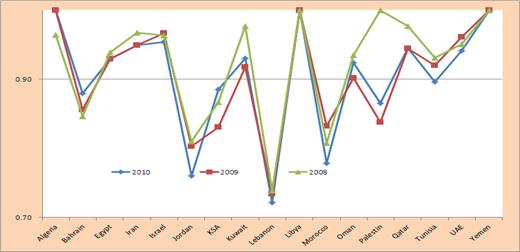
Furthermore, to measure bank efficiency across countries, the efficiency score for all banks is aggregated at country level to get the annual average efficiency scores for each country’s commercial banks. Figure 5 illustrates the results.

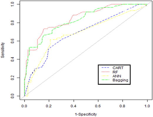
Figure 5 shows the Algerian, Libyan and Yemen commercial banks outperform other countries banks. On the other hand, Jordanian and Lebanese commercial banks performed badly during the study period. The first stage results show the differences in inefficiency among banks in the 17 MENA countries. In this stage, the DEA results are classified into two groups, namely, efficient group (score of 1) and inefficient group (score of 0). This grouping is used as a target variable in each predictive technique. The classification or prediction performances of these techniques are presented in Table V based on the testing data set. It is seen that CIT outperforms the other techniques on sensitivity; however, it produced the lowest overall accuracy (67.55 per cent). RF-CART and bagging show the best overall performance with AUC of 0.9293 and 0.9221, respectively. Moreover, their estimated AUCs exhibit the lowest standard errors (S.E.).

Aside from the numerical measures, the graphs in Figure 6 highlight the comparison between the methods (classifiers) based on ROC curves. The ROC curve is useful for visualizing the overall performance of a classifier. It maps the sensitivity against 1 - specificity. The closer the curve is to the upper left corner, the higher the performance of the classifier. Figure 6 clearly shows that RF and bagging exhibit highest performance, whereas CART, CIT and ANN exhibit the poorest performance. Thus, RF and bagging could be potentially helpful tools for predicting bank performance. However, knowing what factors affect bank performance in MENA countries might be of interest to practitioners. Therefore, RF technique is used to determine the predictors’ importance in the process of predicting bank efficiency

For robustness purposes, we re-estimate the second-stage analysis using linear regression model using the same variables. The justification for carrying out this additional analysis is to compare the result of the best performs data mining techniques with the traditional well-known regression technique. The result of this comparison is reported in Table VI, which overall appear to corroborate the key findings reported in Table V and Figure 7. Specifically, we continue to find that both RF and bagging techniques outperform the regression test. It is worth to note that regression test (LR) shows competitive performance with CART and RF-CIT on overall accuracy and specificity, but it outperforms them on sensitivity.

To identify the most critical environmental variables on bank efficiency and to investigate the interaction between efficiency score and the changes in the environmental variables Table VII reports the results.

Table VII lists the factors from the important of each variable based on RF and the significant variables based on linear regression. As Table VII, shows that both results agreed on the most important and significant variables: country, cost to income ratio and equity/net loans seem to be the most important factors in predicting bank performance, while interbank ratio and loan loss provision/net interest revenue seem to be the least important factors. This means that the performance and steady growth of the financial sector depend on an adequate regulatory framework. It is worth to note that these results are consistent with the findings of recent studies by Wanke et al. (2016), Li et al. (2017) and Sufian (2009) who found positive relationships between bank efficiency and equity to total assets ratio, ROA, ROE, loan loss reverse to gross loan and cost-to-income ratio.

Hence, the major concern of policymakers in countries with an inefficient banking sector need to investigate the reason for this inefficiency and learn from other countries with an efficient banking sector to improve and strengthen their financial sector. They need to understand the mechanisms of a healthy financial environment and help promote the health, safety and vitality of their banking sector in the coming years. The analysis also suggests that the decline in relative technical efficiency was attributed to the following many reasons such as cost-to-income ratio, equity-to-net loans ratio, equity-to-total assets ratio, loan loss reserve-to-gross loans ratio, net loan-to-deposit and short-term funding ratio and equity-to-liabilities ratio. This suggests that strong and prompt policy actions are needed to address these variables and recapitalize bank assets and cost to be more efficient.

Take for example, the cost-to-income ratio is widely regarded as a yardstick when comparing productivity and efficiency of banks, a high cost-to-income ratio is equivalent to low productivity and low efficiency and vice versa (Burger and Moormann, 2008). Also, equity-to-net loans ratio is another important variable of bank efficiency that represent the percentage of the total assets that are financed by stockholders, as opposed to creditors. A low equity ratio will produce good results for stockholders as long as the company earns a rate of return on assets that is greater than the interest rate paid to creditors.

Furthermore, investors will gain more return from investing in MENA countries’ banking sector if they invest their money in those countries whose banking sector is efficient. In addition, if bank managers want to open new branches in MENA countries, they are advised to open them in countries that have a healthy financial environment for the bank to be considered efficient.

Different statistical and data mining techniques have been used in DEA second stage to measure the impact of environmental variables on a DMU performance. Each method has its advantages and disadvantages. Most previous studies of bank performance that use the DEA second-stage approach have focused on how to explain the impact of an environmental variable on bank performance instead of predicting future bank performance. This study focused on comparing seven popular statistical and data mining techniques used in second DEA stage for bank performance to better predict bank performance in MENA countries. The techniques we used comprised CART, CIT, random forest based on CART (RF-CART), random forest based on CIT (RF-CIT) and bagging, as well as ANNs and LR. RFs and bagging have gained popularity in recent years due to their superior performance in a range of applications. However, these methods, particularly random forests based on CIT, have not been used widely to predict bank performance. We provided a comparison of performance considering several measures of prediction performance such as sensitivity, specificity, overall accuracy and the area under the ROC curve (AUC). Approximately, the seven methods showed adequate ability to model bank performance. However, the overall performance of random forests and bagging was superior. A key advantage of random forests is also the variables importance ranking. In our case, RF ranked “Country”, “Cost to income ratio” and “Equity/Net loans” as the most important factors in predicting bank performance and “Interbank ratio” and “Loan loss provision/Net interest revenue” as the least important ones. We agree that any specific data may have different fits from different data mining techniques. In the context of bank performance prediction with a target variable (Efficiency) obtained from DEA-VRs (which is our case); RFs based on CART trees were powerful tools to predict bank performance in MENA countries. Therefore, they would be of a great benefit to practitioners and researchers in MENA countries who are interested in predicting bank performance.

The result shows that both RFs and bagging techniques are the best tools to predict bank performance using DEA-VRS model. Future research should target different data set and carefully analyze the role of their environmental and regulatory specifics in efficiency levels with other DEA models such as slack-based measure and network DEA, to predict the efficiency of DMUs. However, the availability of real data is challenging; thus, a study involving simulations of different scenarios could be an interesting topic to be explored. Furthermore, as data mining tools are sensitive to used data; hence, possible venues of future studies could also try to overcome some limitations of the current study by using other environmental variables other the one used in this study to test the robustness of RFs and bagging techniques in predicting performance.