The alignment of global equity and corporate bonds markets with the Paris Agreement: A new accounting framework

The Paris Agreement (PA), adopted in 2015 and effective as of November 2016, defines the global political commitments on climate change (United Nations Framework Convention on Climate Change, 2015). Specifically, Art. 2 of the PA defines the ultimate aims of the framework, namely:

A significant body of literature and policy initiatives has been dedicated to and emphasizes the first two sub-articles on climate mitigation and adaptation. The PA also elevates the alignment of financial markets as a core political commitment. Decarbonization scenarios, such as those published by the Inter-Governmental Panel on Climate Change (Intergovernmental Panel on Climate Change, 2017; Integrated Assessment Modeling Consortium, 2017) or the IEA (2016a), do not specifically cover trends in the financial sector. The translation of economic transition trends into financial markets is missing.

At the same time, there is a growing demand both in the public and private sectors for what can be labelled 2°C scenario analysis in financial markets; analysis as to progress on Art. 2.1(c) of the PA. 2°C scenario analysis is generally considered the most critical and innovative aspect of the disclosure recommendations developed by the FSB TCFD (2017). It also forms the basis of voluntary disclosure pilots led by governments and private sector actors (e.g. Switzerland Climate Compatibility Pilot). 2°C scenario analysis and target-setting also form the basis of the first mandatory climate disclosure framework for investors in the world, Art. 173 of the French Energy Transition law 2015 (Legifrance, 2015).

This paper seeks to respond to both the political demand for understanding progress on Art. 2.1c and the demand in the private sector for understanding trends at the portfolio level. Specifically, it provides a methodological framework to translate economic decarbonization scenarios into benchmarks for listed equity and corporate bond markets and portfolios. The model presented here builds on the methodological frameworks piloted in the EU H2020-funded Sustainable Energy Investing metrics (SEIM) project, applied to date by over 200 financial institutions, as well as a number of financial supervisory authorities and governments (Thomä et al., 2015, 2017). It provides a summary methodological documentation of the model and accounting principles underlying the work of both of these projects.

The paper represents the summary findings of the methodological development of a 2°C scenario analysis framework that seeks to measure the alignment of financial portfolios with climate goals. Specifically, it builds on the lessons in applying the model with over 250 institutional investors, the Swiss Government and two financial supervisory authorities. The paper summarizes the core accounting frameworks distilled from these applications, as well as the differences in approaches chosen by different stakeholders. It represents the first general accounting framework responding to the question of measuring the alignment of financial portfolios with climate goals, specifically focusing on portfolios associated with corporate issuers of debt and equity.

The paper is organized as follows: Section 2 provides a review of relevant literature concerning portfolio alignment with the transition to a low-carbon economy, Section 3 discusses the relevant data required for scenario analysis in the context of climate change, Section 4 walks through the accounting principles of utilizing these data sources for scenario analysis, and Section 5 provides current formulations used by financial supervisory authorities and governments as well as an outlook for future analysis for other asset classes. The paper concludes with a discussion of limitations in Section 6 and concluding remarks in Section 7.

The framework presented here seeks to build a calculation rule around an optimal investment theory under a non-financial constraint – specifically the goal of aligning the portfolio with the transition to a low-carbon economy. The point of departure for the literature review then is traditional modern portfolio theory and alternative frameworks.

The origin of modern portfolio theory is the seminal work “Portfolio selection: efficient diversification of investments”, where Henry Markowitz, its author, develops a mathematical relationship between risk and returns, showing that the expected return of a portfolio is the weighted average of the expected return for each security. Volatility risk (standard deviation) sums to less than its weighted average if the correlation between securities is less than absolute (Markowitz, 1952). Markowitz goes on to argue that portfolios that maximize return while minimizing risk sit on the efficient frontier^[1].

Building on this theory, James Tobin built on the work of Markowitz by coining the concept of the “super-efficient portfolio” – the portfolio everyone should hold in combination with a risk-free asset (e.g. cash) (Tobin, 1958). The ratio between the risk-free and super-efficient portfolio would then be determined by the risk averseness of the investor. His theory is also known as the “separation theorem”. Tobin thus took the intellectual leap from investment to portfolio theory to the dawn of modern asset allocation^[2].

To appreciate the dynamite contained in these ideas, it is critical to marry them with a parallel strand of thinking being popularized at around the same time, namely the efficient market hypothesis, which concluded that if market prices integrated all available public information about any individual security, it would be impossible to systematically “beat the market” as an investor, except by luck, circumstance, insider knowledge or some combination of the above. The first formal argument for this idea can be found in Samuelson (1965)^[3], who showed that studying historical prices for forecasts is an exercise “doomed for failure [as] the market has already discounted all knowable future information”. It is relevant here to note that Samuelson did not conclude that the market prices were not always correct, but rather superior estimates to alternatives. Today, the efficient market hypothesis is most popularly associated with Fama (1965) who in his paper on the behaviour of stock market prices coined the term, defining it as “a market where, given the available information, actual prices at every point in time represent very good estimates of intrinsic value”.

The growth of passive investing is arguably a function of the growing consensus that market actors cannot beat the market, given its “random walk” characteristics (PWC, 2014). Modern portfolio theory, as developed by Markowitz (1952), Tobin (1958), Sharpe (1964) and others, relies on the assumption that optimal investing strategies involve adopting market assumptions around prices and diversifying portfolios accordingly.

The combination of the efficient market hypothesis and the vision of the modern portfolio theory launched by Markowitz culminated in the capital asset pricing model (CAPM) of Sharpe (1964), who suggested that Tobin’s super-efficient portfolio was in fact the market portfolio, given that the market provided the best available evidence of prices.

In the CAPM, Sharpe suggests that there are two types of risks: systemic risk, i.e. market risk (called beta), which is contained in all securities, and idiosyncratic risk (alpha), i.e. risk specific to an individual security. In other words, when prices of an individual security go up as market prices go down, this is the manifestation of alpha. When an investor buys the super-efficient market portfolio, he or she eliminates all idiosyncratic risk. It should also be noted that it is well established that it is impossible to create such a portfolio as it would require capturing every convincible investment opportunity (Roll, 1977).

In addition, the CAPM has a number of relatively strict assumptions and comes with a glaring paradox; it requires homogenous investors with identical return expectations and investment horizons, no transaction costs or taxes, unlimited liquidity, borrowing and lending at risk-free interest rates, all investors seeking to maximize return and minimize risk, and asset returns that are normally distributed.

The equation summarizing the premise of CAPM can be summarized as follows (Sharpe, 1964), and can also be extended to a firm-level analysis:

where E(R_i) is the expected return on the asset, R_f is the risk-free rate, β_i is the sensitivity of the returns to the expected excess market returns and E(R_m) is the expected return of the market.

CAPM remains the most dominant theoretical force in portfolio management to this day. Adjusted, abridged, but never abandoned, it continues to inform how the largest pension funds and insurance companies invest their beneficiaries’ money.

Most adjustments and further developments of CAPM assume some types of “factor” that allows for outperformance above and beyond simply buying the market. Thus, Black et al. (1972) show that “portfolios constructed to have zero covariance with the market had average returns that significantly exceeded the riskless rate which suggests that there is (at least) another factor besides the market that systematically affects the return on securities”.

A range of academics since the 1960s have been able to demonstrate other factors beyond beta acting as predictors of return, notably low price-to-earnings ratios (Basu, 1977), low book-to-market ratios (Chan et al., 1995; Barber and Lyon, 1997), leverage (Bhandari, 1988) and short-term price momentum (Jegadeesh, 1990). When integrating the assessment of bonds, Fama and French (1993) developed a three-factor model (FF3) and then a five-factor model (1996)^[4], that, the authors claim, ultimately unifies these model advances based on the simple idea that CAPM works, albeit with morethan just a market factor (Fama and French, 2004). Naturally, there remains a range of fundamental criticisms to a factor approach, notably based on the idea of market inefficiency (Rosenberg et al., 1985).

To date, the interface between climate change and finance largely builds on this literature, turning the transition to a low-carbon economy as one potential “mis-priced” factor that allows for outperformance. The theoretical framework for why these types of risks are mis-priced has been developedby Thomä et al. (2015), arguing that these risks fit into the traditional categories that drive market inefficiencies (e.g. satisficing behaviour, hyperbolic discount functions and institutions). Andersson et al. (2016) developed a climate risk factor approach to design low-carbon products designed to outperform traditional market portfolios under the transition toa low-carbon economy. Coeslier et al. (2016) in turn highlighted the need to move beyond simple to multi-factor frameworks within transition risks.

The accounting framework developed here takes an alternative approach. Rather than seeking to introduce a factor into the traditional CAPM, it provides for a restatement of the market portfolio more generally. It does not seek to “tweak” the portfolio based on a given factor, but rather design the market portfolio as it would look under a 2°C transition and based on this benchmark calculate the deviation of a given portfolio from what can be labelled the 2°C market portfolio. The analysis builds on the development of alternative optimal diversification concepts developed previously (Thomä et al., 2015, 2016) that are here being applied for the first time in a rigorous accounting framework.

The authors acknowledge that the corporate debt and equity markets only capture a portion of available investment opportunities within the global capital market; credit, sovereign and municipal debt and private placements play a substantive role in the operation of capital markets that finance the greater economy. Beyond data accessibility limitations, arguments to why these cannot be incorporated within this type of methodological framework are few. Nonetheless, it must be acknowledged that to accurately capture risk associated with the misalignment of the capital markets with the climate commitments, all financing mechanisms need to be included.

The translation of economic transition trends into financial markets requires four types of data: scenario data; economic activity data; financial market and ownership data, and lastly, if trying to measure the trend of a specific financial actor; iv) financial portfolio constituent data. This section will walk through of each of these different data needs individually.

Energy transition scenarios detail the potential decarbonization of the global economy. This is done through use of integrated assessment models of global economies and climate systems that provide potential pathways for global energy production and broader climate-related industrial trends. These pathways are underpinned by projected global macroeconomic trends, modelled climatic response to the associated greenhouse gas concentration and the potential resultant global warming. These data are published primarily by the Integrated Assessment Modeling Consortium and used to drive projections/pathways of industry production capacity from different technologies under scenarios that represent certain probabilities on maintaining global temperatures with some threshold, such as 2°C. These potential production pathways in turn are published by the likes of the International Energy Agency (IEA), Greenpeace and industry actors (e.g. Shell, BP), and it is this level of modelling that can inform scenario analysis.

The specific choice of scenario is not fundamental to the framework provided here; indeed, the framework should be able to process a range of different scenario inputs. What is of crucial importance, however, is that whatever choice of scenario is applied, the unit of accounting within that choice is consistent with the unit of accounting used in the economic activity data that inform the comparison of the financial portfolio to the scenario. Thus, if the analysis is conducting 2°C scenario analysis on production capacity, for example, the scenario units need to be expressed in this way.

Economic activity data, or “climate data”, are required to identify a financial actor or markets’ alignment with, or exposure to, the economic activity that can be associated with 2°C scenarios and inform on associated financial analysis. It can be used as a reference point in the context of the allocation of macroeconomic scenario data to microeconomic actors. There are a range of different economic data points that can be sourced to define the climate unit of a firm, u^issuer, and can be accounted at four levels: the physical asset, business activity (sectorial), the firm and the market sector. Depending on data availability in the market and the type of analysis desired, different levels may be more or less appropriate (Thomä et al., 2018).

When it comes to sourcing economic activity data, with the exception of R&D, which can only be quantified at the company level, the key underlying data defining a company’s activities begin from the individual asset level. The discrimination of individual assets allows for a regional benchmarking of the analysis to regional scenarios (where those exist, e.g. for power production) and a direct link between economic activity by technology and sector to the scenarios. It also enables the assessment of granular physical transition risk and policy risks.

This individual asset-level data can come through aggregated corporate reporting channels or through asset-level databases that collect data from a range of sources, including press releases, regulatory filings, surveys, annual reports and industry publications (Weber et al., 2017). The actual choice in terms of data sourcing is independent of the application of 2°C scenario alignment analysis, that is to say both options are in theory acceptable. In practice, however, asset-level data are significantly more suitable. Corporate reporting at the physical asset level is often inconsistent in terms of timeliness of disclosure, accounting principles and coverage in terms of both geography, and type of asset and/or reporting entity (Dupré et al., 2015; Raynaud et al., 2015). This limits the universal applicability of the scenario analysis itself, and thus can undermine its role of providing market or global prospectus. On the other hand, asset-level database created by market intelligence organizations allows for more comprehensive scenario analysis for typical financial portfolios due to possible standardization and choice of accounting rules, being actively maintained, and often including forward-looking activity (Weber et al., 2017; Caldecott and Kruitwagen, 2016).

That is of course not to say that this type of data does not have its shortcomings (Table I). Primarily, these relate to the lack of transparent formal auditing of the underlying data, which lead to different databases having conflicting information on the ownership of a given asset. In addition, the data sets can be limited to particular industrial sectors, and are not necessarily harmonized across different business activities, making consolidation for diversified firms or large corporate entities expensive and technically difficult to undertake. To the authors’ knowledge, the assessment of the quality of the asset-level data corporate information has only be undertaken in one study (Glattfelder and Hayne, 2017), and no formal cross evaluation of asset-level database has been carried out to date.

As outlined above, for 2°C scenario alignment analysis, the climate units need to be expressed in the same unit as the scenario itself for comparability. Thus, the data point may either be expressed in production capacity, production, investment/financing and/or CO₂/GHG emissions. The choice of indicator among this category is somewhat subjective and involves various trade-offs, summarized in Table II.

Given the balance of pros and cons, the SEI metrics project relies on the production capacity logic, organized either by CO₂ intensity or technology. The reason for this is that it minimizes the data uncertainty in the economic activity data, can be linked to equivalent units in the scenarios that have lower uncertainty than investment levels, and reflects the “supply decisions” that companies control. While this is the choice taken in these methodologies, alternative choices can equally be deployed using related conversion factors, with the exception of the use of production capacity data relating to R&D investment figures, where investment figures need to be mobilized.

The third and fourth piece of the data analysis, respectively, is the financial portfolio and financial data. With regard to financial portfolio data, this is of course a function of the organization or individual applying the analysis and can extend to a series of financial portfolios at the institution level – in the case of application by financial supervisors – to individual funds of asset managers. Financial data in turn are needed as a function of the exact model calibration and thus its use will be discussed in the next section discussing the model construction.

The analysis provided here builds on the models developed in the EU funded SEIM. A variant of these models has been applied by over 200 financial institutions in their portfolio analysis, as well as two financial supervisory authorities and the Swiss Government. This section walks through the general principles of the equations used for scenario analysis, starting with basic fundamental equations, the units of measurement, the allocation of units to financial instruments and the benchmarking process against scenario pathways.

In the course of application with financial institutions, two different approaches materialized, which are summarized in the equations below. It is worth briefly highlighting each in descriptive terms. The first approach suggests measuring the 2°C alignment of a financial portfolio at some future points t relative to what is here called a “2°C benchmark”. This approach is basically an extension of traditional tenets core to modern portfolio theory, where future optimal diversification is not measured with regard to a financial, but rather a climate-related target. This approach involves measuring the delta of the aggregate portfolio exposure to a climate unit, u^x, with the market exposure under a 2°C transition. The market exposure under a 2°C transition here represents the expected evolution of the defined market, which can be scoped in various ways similar to the application of different traditional benchmarks (e.g. equity market, economy, regional equity market, a set of peer portfolios), under a 2°C transition.

The second approach can be labelled as the “trajectory approach”, where the measurement does not compare absolute exposure at a future point to the absolute exposure of a market benchmark, but rather seeks to compare two rates of change, namely the rate of change in the portfolio with respect to the climate unit, and the necessary rate of change under a 2°C transition.

The basic equations governing the two approaches can be summarized by the following equations for a portfolio, although the concept can also be extended to a firm-level analysis:

where u represents a climate unit defined as one of three key climate metrics based on the taxonomy developed by Dupré et al. (2015). These three units are either GHG emissions, green/brown metrics (i.e. low-carbon or high-carbon products and services) or qualitative scores, depending on the choice of economic activity and scenario data discussed above. In principle, while the focus here is on financial portfolios, the climate unit can either be calculated at company level (u^issuer), individual portfolio level (u^port) or for a group of portfolios (e.g. the listed equity market in aggregate, u^market). In turn, u^bench represents the value that u should take to be consistent with a target climate outcome/the scenario. Thus, when applied in conjunction with a 2°C climate goal, it is designed to reflect a benchmark exposure consistent with the Paris Agreement objective.

The specific configuration of these two fundamental equations will now be broken down in further detail.

The portfolio’s climate unit, u^x, can be calculated as follows:

where p is the value of instrument i in a portfolio with a total of f instruments, a is the allocation factor that allocates the economic activity of the instrument i to the portfolio u^issuer is the climate unit of the issuer of instrument i, and n is the normalization factor in those cases where the climate unit of the company is normalized in some form.

The logic of the equation can be explained as follows. Defining the climate unit of the portfolio requires allocating the climate units associated with the issuers of the instruments within the portfolio by some fixed rules to the portfolio. This allocation factor is a function of both the value of the issuer’s instrument in the portfolio and some factors that determine how that weight should be put into context. One simple factor here is the total weight of the portfolio, basically creating an allocation factor that distributes the climate unit of the issuer to the portfolio as a function of the percentage that the associated instrument represents in the portfolio. The calibration of this allocation factor will be discussed in further detail below.

For sake of completeness, a normalization factor is added since the climate unit may be normalized in some cases. One simple example where normalization may be relevant is where the portfolio climate unit is meant to represent a weighted GHG emissions intensity of power production, for example. In this case, the climate unit of the issuer needs to be total GHG emissions over total power production, where total power production does not actually represent a climate unit, but a normalization factor by which the climate unit is normalized and thus set in relation to another unit (in this case, power production). On the other hand, comparing absolute ownership of renewable power between two portfolios would not require a normalization. By extension, the use of this normalization factor is a function of the exact analysis desired.

The allocation factor is determined by the analysis approach, to which here we consider two fundamental types: the balance-sheet approach (a^bl) and the portfolio-weighting approach (a^wt). Again, it is relevant to first describe the logic of the two before diving into the equations. In simple terms, the balance-sheet approach allocates the climate unit of the instrument of the issuer as a function of how much the portfolio owns of all outstanding instruments of the issuer. This approach can be said to represent a “responsibility” logic. As will be outlined in further detail below, the responsibility can be a function of the portfolio ownership in all outstanding instruments in that asset class (e.g. equity ownership) or take a broader view. The portfolio-weight approach in turn allocates climate units based on the share of the instrument in the portfolio, creating a weighted climate unit as a function of the capital that was allocated by the portfolio to different instruments. The key difference between the approaches is the allocation through portfolio weighting, which is defined solely by the construction of the portfolio, while the balance-sheet approach considers the relative volume of each instrument in the portfolio alongside the respective size or value of the firm or asset class. The equations governing each approach are summarized as:

where g represents the number of instruments in one asset class, and h represents the total number of asset classes issued by the firm or held in the portfolio under evaluation.

For example, in the case of assessing equity with the balance-sheet approach, a^bl can represent the outstanding equity of firm i, being the sum of all equity over each equity instrument, g, issued by the issuing firm of instrument i. Thus $pi/aibl$ is then equal to the ownership share the portfolio has in the issuer, and the product with $uiissuer$ represents ownership of the climate unit of the issuer of instrument i. Finally, u^port then represents the total portfolio ownership. The concept of issuer can also be extended to all financial instruments, such that a is equal to the enterprise value of the firm, or another subset of outstanding assets (e.g. long-term debt plus equity).

The key challenge with this allocation factor is that when it is extended outside of equity, where ownership percentages can be calculated independent of financial asset price movements, price biases can be introduced related to the movement in asset prices, which in turn introduce fluctuations in the metric that are not necessarily correlated with changes in capital expenditure or production plans. This can follow on to introduce bias and uncertainty around the required action of the portfolio owner or manager. In the case of enterprise value, this fluctuation is driven by changes in relative market prices (Thomä et al., 2018).

The alternative portfolio-weighting approach, a^wt, calculates relative intensities of the portfolio’s exposures to different products and services, rather than the desire to measure absolute ownership. As the allocation is based off the relative value of each instrument in the portfolio alone, portfolios across asset classes can be jointly examined. Here, only one type of option can be considered, namely the overall size of the portfolio.

It should be noted that intuitively, the absolute units calculated using the portfolio-weight approach may not be meaningful. For example, a portfolio that exclusively owns an oil and gas issuer will be allocated 100 per cent of the climate unit of said issuer, even if the portfolio size is only $100. At the same time, sectoral weighting approaches described in further detail below can contextualize the figure with a benchmark to highlight the relative intensity of the exposure. Equally, in the case of the power sector, relative renewable power intensities of different companies can be weighted using the portfolio-weight approach to highlight the capital allocation choices of the portfolio manager.

In summary, the framework described until this point looks at how to calculate the climate unit of the portfolio. The next section will discuss how this climate unit can be benchmarked in the context of 2°C scenario analysis.

The benchmark, $utbench$⁠, has to be expressed in the same climate unit as $utx$⁠, and is calculated as follows:

where s represents the starting point of the benchmark when t = 0, and e_t the decarbonization pathway, i.e. expected change to s at time t in order to be consistent with the 2°C climate goal. s can be calculated in three different ways, depending on the desired normalization of the portfolio, as shown in Equations (8), (9) and (10):

where j is the number of instruments in the market:

where $ut0port$ and $ut0market$ is the initial aggregated climate unit for the portfolio and market calculated through Equation (4), respectively, which is summed over the number of each technology represented in the market, k, and the portfolio, l:

where m is the number of instruments in the portfolio from issuers classified under a specific business activity/sector, with n the number of instruments from all issuers classified under the same specific business activity/sector within the market.

While all three options can be applied, the choice between one or another relates to both the sector and the objective of the analysis. Equation (8) calculates whether the portfolio over- or under-weights a climate unit in absolute terms, independent of the exposures to other climate units. It may thus be more relevant for sectors and products where the scenario itself makes a comment on the evolution of the business activity itself. For example, in the case of fossil fuels (oil, gas and coal production), 2°C scenario generally suggests a decline of absolute production capacity over time, and thus a decline of the value of a portfolio or firm derived from that sector and calls for a production intensity-based metric.

As in illustrative example, consider the application of Equation (8) for a portfolio with a portion of investment in equity from the coal sector, and it is to be evaluated using the balance-sheet approach with no differentiation on the type of coal produced. In this case, u^market calculated via Equation (4) in conjunction with Equation (5) would yield the total production of coal from all firms in the market. s^p would then be the production of coal allocated to the portfolio at the initial point in time based on the current intensity of coal production of the equity market. At this initial point in time, this allocation would be synonymous with comparing the portfolio to a completely diversified equity portfolio, owning the same portion of coal production per asset under management, as the equity market as a whole.

For sectors where the evolution of the business activity is considered “neutral”, and the modelling pathway makes comment on the different technologies and production processes within the sector, considering the weight of climate units in the sector may be more relevant, i.e. though Equation (9). For example, in the case of the power and automobile sector, while the different scenarios assume different aggregate levels of production capacity over time, the key driver of the scenario is the switch from high-carbon to low-carbon fuels in the case of the power sector, and the switch from high-carbon to low-carbon powertrains in the case of the automobile sector. In this environment, it may be relevant not just to understand how high the exposure of the renewable power generation to total electric power is, but also the weight of renewables to coal-fired power in the portfolio.

As in illustrative example, consider the application of Equation (9) for a portfolio with a portion of investment in equity from the power sector, and it is to be evaluated using the balance-sheet approach. In this case, u^market calculated via Equation (4) in conjunction with Equation (5) would yield the total production capacity for each of the power-generating technologies represented in the equity market’s power sector. s^u would then be the production of each of these technologies allocated to the portfolio at the initial point in time, based on the share of the power market the equity portfolio owned at time t₀.

The choice for s^sec, given that it is a rougher sector proxy, appears as a second-best solution where the other two options cannot be applied for technical reasons without creating biases, for example in the case of calculating a starting point for the fossil fuel production capacity in corporate bonds portfolios when applying the portfolio-weight approach.

To calculate the required change to the benchmark, e_t is defined as follows:

where:

where $utscenario$ represents the economy-wide climate unit (e.g. production capacity associated with a specific product or service, e.g. renewable power capacity) as prescribed by the decarbonization scenario, and c is a constant to describe any adjustment of the market share over time. This could be important in business sectors where market share between economic agents is predicted to change over time. For example, the case of renewable power generation, where in some regions household owned power capacity has been broaching on the utility power market due to the differentiated responses of both participants to certain government incentives. In this case, c_t could be used to account for the continuation of historical trends, and explicitly in this example, account for the reduction of listed utility power overall market share of total renewable power.

The analysis is somewhat complicated by the fact that for low-carbon technologies, it may be relevant to disentangle the market share in the technology and the market share in the business activity more generally. Thus, if a utility, for example, has 10 GW of electric power capacity, but zero electric power, simply taking the market share in renewable power (in this case, zero) would suggest that such a utility would not be expected to build out renewables. This is prime facie absurd, since such a strategy would allocate full responsibility for capacity additions to historical leaders and absolve historical laggards (not to mention imply a decline in overall market share over time). On the other hand, an electric utility that owns 10 GW of electric power, but no coal-fired power would not be in a position to retire any coal-fired power. This dichotomy between high-carbon and low-carbon technologies requires a calibration of the model to reflect this distinction.

To resolve this tension, the model controls for whether the climate unit, u^x, is associated with a high-carbon or low-carbon product or service through an extension of Equations (11)–(13):

where:

and:

where $utx,sector$ and $utmarket,sector$ represent the total volume of $utx$ and $utmarket$⁠, respectively, across all products and services in one business activity for the portfolio and the market (e.g. the sum total production capacity, in MW, across all types of power-generating assets – renewables, coal, gas, etc.), and d is a dummy value which takes the value 1 if u is associated with a high-carbon product or service and −1 if u^x is associated with a low-carbon product or service.

The previous section discussed the modelling framework and equations underlying 2°C scenario analysis. In this section, the choices for application for two specific use cases will be discussed in further detail: the Swiss Government and a financial supervisory authority. Given confidentiality, the name of the financial supervisory authority cannot be revealed at this stage.

In Switzerland, the Swiss State Secretariat for International Financial Matters (SIF) and the Swiss Federal Office for the Environment (FOEN), together with the 2° Investing Initiative, initiated a voluntary pilot project in 2017 to analyse the alignment of Swiss pension funds and insurance companies with the Paris Agreement. As part of this pilot, 79 Swiss pension funds and insurance companies, representing around two-thirds of the market (measured in share of assets under management of the sector), participated. The project limited its analysis to the investors’ listed equity and corporate bonds portfolios. The project involved a meta-analysis for the Swiss Government and tailored individual reports for the participating investors.

In terms of data sources, the IEA scenarios were chosen, notably Energy Technology Perspectives for the transport and industrial sectors, and the World Energy Outlook for the fossil fuel and electric power sectors (IEA, 2014, 2016a, b). Since IEA data are presented in five-year intervals, data are interpolated using a linear function where required. Data for the scenario pathways are extracted with a 25-year time horizon. Scenario data are extracted for the regions provided by the scenario provider. This allows for a regional assessment if desired in terms of regional alignments with scenario trends.

The value of the financial instruments in individual funds and in the listed equity market was taken from Bloomberg with data current as of the end of the 2016 calendar year. Bloomberg is also the data source that allows for a definition of the market size. The total listed equity market size is derived from Bloomberg data. Crucially, the listed equity market portfolio only includes the free-float share of a company’s equity value. This is done to distinguish the investable universe (free-float) and by extension derive a benchmark for the investable universe, rather than the economy as a whole. There are a couple of implications worth highlighting notably that the total climate units in the listed equity market or corporate bonds market are not equal to the total climate units in the economy (given household ownership and ownership by companies that do not issue financial instruments). One concrete implication in practice is that the renewables unit weight in total power is lower in listed equity markets than in the economy since the economy also includes households, which have a renewable power “bias” relative to power assets owned by companies.

In the model calibration, p_t is always fixed – even if instruments mature at point t<5, at t=0 in order to provide for a consistent analysis. This assumption can of course be adjusted such that p₅ is considered, if desired. The underlying choice will then inform the data needs from Bloomberg and the portfolios.

The meta-analysis applied the trajectory exposure approach highlighted above (Equation 3), focusing on an analysis of the rate of change. In applying the trajectory exposure approach, it looked at absolute changes in production capacity across the energy, power and automobile sectors as the three sectors with the most significant climate impact in Swiss pension funds and insurance companies listed equity and corporate bonds portfolios. Climate units in the portfolios of Swiss pension funds and insurance companies were allocated using the portfolio-weight approach for corporate bonds and the balance-sheet approach (based on equity ownership for listed equity). The choice of two different allocation rules for different asset classes was based on the following reasoning: given that the objective of the analysis was to identify a responsibility as a point of departure for climate impact, using the balance-sheet approach appeared as the more appropriate allocation rule in general. However, the price and financing biases in corporate bonds markets make this approach somewhat unwieldy and potentially subject to significant biases, as outlined above. As a result, the preferred allocation rule was applied where possible, with the resorting to second-best for corporate bonds. No normalization factors were considered, with each technology and production capacity estimate treated individually.

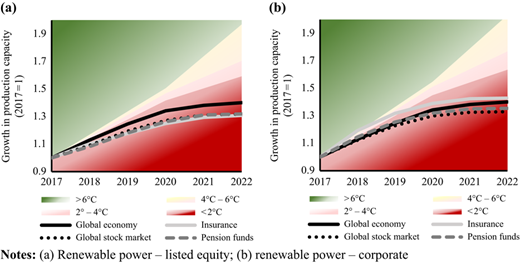
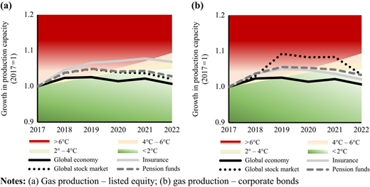
Figure 1 shows the results for renewable power and gas production (Thomä et al., 2017). It is relevant to note here that the results are not represented as percentages, but as line charts. Relating this to the equations discussed in the previous section, Equation (3) can be traced here in terms of comparing the start and end point of each line in the chart to the start and end point of the demarcation line between the green and yellow space, the difference representing the misalignment with the 2°C scenario as expressed in the trajectory approach (Figure 2).

While the Swiss Government focused their analysis on the trajectory exposure, Swiss investors were provided the results for Equation (1) in their individual reports. Here, the same allocation rules were chosen as for the trajectory approach. Consistent with the different roles that fossil fuels play relative to the automobile and power sector in the scenario, the starting points for fossil fuels were based on Equation (9) and for electric power and automobile on Equation (8).

In order to create a consistent scale where outcomes larger than 1 always signify a positive exposure and outcomes smaller than 1 always signify a shortfall, a dummy variable d can be added to the equation which takes the value 1 when u accounts a high-carbon product or service and −1 when u is associated with a low-carbon or zero-carbon product or service. This variable, however, simply helps to homogenize the result in a way that is more easily understandable for users and is not core to the equation, in particular where the result is expressed in GHG emissions, where the low-carbon/high-carbon distinction does not exist. Adding this factor complicates Equation (2) somewhat, but ensures more intuitive results, such that:

The new equation added the dummy variable and turned the equation into an absolute value equation to avoid negative results, as well as range constraints to avoid the dummy variable influencing the underlying results. The range constraint caps the value of $ut+nport$such that it does not exceed $2ut+nbench$⁠. The constraint limits the results to 0⩽y_t+n⩽2, allowing for a consistent and intuitive explanatory power of the results, albeit at the expense of hiding outliers captured in Equation (2).

The application described above in the case of the Swiss pilot project was motivated from the perspective of measuring the alignment of financial flows with the Paris Agreement. An alternative application is that explored by financial supervisory authorities seeking to conduct 2°C scenario analysis more from a risk perspective. The logic motivating such an analysis relates to two types of research questions relevant from the perspective of a financial supervisory authority. First, to what extent does the misalignment of financial flows with climate goals may create future financial volatility should climate policies and market trends adjust. Tracking the investment and production plans in financial markets (and portfolios) helps to inform on this question and allows financial supervisory authorities to potentially anticipate and where appropriate explore ways to respond to future volatility. The approach highlighted in the previous section explored by the Swiss Government incidentally addresses exactly this question.

At the same time, there is a second question that derives from this issue, namely the scale of exposure should such risks materialize. This second question requires an alternative approach than the modelling calibration applied in the Swiss project across the range of modelling choices described above. The application described here is that of one pioneered by one financial supervisory authority in Europe in the context of conducting 2°C scenario analysis of their regulated entities, notably focusing on insurance companies.

The pilot project in question, with results set to be published in the second quarter of 2018, used the portfolio data of insurance companies that they regulate. European supervisors have been put in a capacity to analyse the insurance data following the implementation of the Solvency II Directive, which among other things mandates the reporting of portfolio constituent information of insurance companies to their financial supervisors. Tapping into this data allowed the financial supervisor to conduct the 2°C scenario analysis described above.

Following the analysis of financial flows, the financial supervisory authority then posed a second question, namely the share of the insurance companies’ financial portfolio that may potentially be exposed to financial disruption – and comparing that share to the expected exposure under a 2°C benchmark. This approach built on the same type of data (economic activity data, IEA scenario, Bloomberg financial data), described above. Instead of representing the results in terms of percentage, however, the climate unit of the portfolio was directly compared – in absolute terms – to the climate unit of the benchmark.

The application concretely involved the following application of the model: following the logic of quantifying the exposure as a percentage of the portfolio, the climate unit was allocated to the portfolio based on the portfolio-weight approach. Climate units were normalized such that the climate unit of an electric utility was derived by taking the percentage power share by fuel source. For example, the climate unit in this case would be installed renewable power capacity, with the normalization unit equivalent to the total installed power capacity of the utility. For oil and gas, oil production capacity was normalized over all energy production of the company.

This allowed for the breakdown of the portfolio into “high-carbon” and “low-carbon” shares, where a 1 per cent exposure to a utility (portfolio-weight) would then for example be converted into a 0.5 per cent renewable exposure and 0.5 per cent coal power exposure in the case where the utility behind the 1 per cent exposure had a fuel mix evenly split between coal and renewables. This approach sought to create a proxy to isolate the part of the exposure that was exposed to the transition to a low-carbon economy generally and the parts of the portfolio that were exposed to such a transition on the high-carbon side.

The benchmark was calculated on the same principle, seeking to quantify whether the exposure of the regulated insurance companies exceeded that of the market and – more specifically – the expected future exposure of the market under a 2°C transition.

The approach provided for a framework to contextualize the potential risks should future economic disruption associated with a more shock-like adjustment to a 2°C transition following continued investment in business as usual translate into financial risks. The results can be compared then to exposures typically identified, for example, in stress-test shocks for listed equity markets or other asset classes. At time of writing, the final results have not been published, although publication is planned in the second quarter of 2018. Illustrative results can thus not be presented here. Equally, the discussion of the modelling framework shows that the general modelling framework developed in Section 3 can be applied both for two very different use cases (alignment of financial flows vs exposure to transition risks) and using different and use-specific articulations.

While it is important to highlight that different use cases also imply low comparability between the results of the two different pilot applications, they demonstrate the power of a common framework that allows different actors to speak the same language when modelling and thinking about 2°C scenario analysis. They also highlight that conscious accounting choices are not just a function of artificial accounting choices, but directly linked to the question being explored in the analysis. For example, the portfolio-weight approach was taken as the more appropriate approach choice for the financial supervisors, vs the balance-sheet approach chosen by the Swiss Government.

The model presented here represents an attempt to create an accounting approach to measure the alignment of financial portfolios. In applying this approach with over 250 financial institutions and a number of policy actors, it is designed to complement existing portfolio management approaches through the introduction of non-financial objectives. It is important to highlight the limitations of the approach presented in this paper.

The first and perhaps most prominent limitation is the incomplete scope of analysis in terms of defining the market. In line with Roll’s critique of modern portfolio theory, the actual market portfolio is unobservable. Within the assessment conducted here, the results are only shown for renewable power assets and gas. While the model can – and indeed in practice is expanded to other sectors^[5], it does not cover the total universe of assets that may be relevant in this regard. While a limitation, the approach does go some way as to lifting the veil on the “unobservable market portfolio” by extending traditional concepts of “asset” from a purely financial to a broader economic description, as well as identifying firms not just as firms, but as the sum of their assets.

Another limitation in the approach presented here is the uncertainty around the benchmark scenario that is being applied. While this is not a shortcoming of the underlying accounting model, it is a challenge in the actual application as there is a limitless number of combinations of economic pathways consistent with specific carbon budgets, which in turn face uncertainty as to the temperature warming they are associated with.

More broadly, the concept of alignment in this paper is framed with regard to a logic of diversification – in the spirit of modern portfolio theory, but in opposition to a “factor-based” approach that reduces diversification as a portfolio strategy benefits from the deployment of a specific factor. This approach, however, is of little value to “value investors” with concentrated portfolios who are not seeking to diversify risks, but rather see investing as a bottom-up approach in the spirit of the original theory of investing of Benjamin Graham and David Dodd, first released in 1934, Graham and Dodd (2009), Williams (1938) and others.

Finally, the approach and analytics presented here are explicitly not a risk quantification approach. While not by default a limitation – as it does not frame the objective of the paper – it is critical to highlight that the accounting framework developed here does not provide explicit quantitative insight into financial or economic risk, but rather a broader suite of questions related to the correlation between asset classes, different discount rates, etc. However, insights gleaned here may be used in future research to inform alternative discounted cash flow modelling, as explored by some equity research analysts, notably Kepler Cheuvreux. This then speaks to broader issues of alternative heterogenous discount rates related to climate futures.

This paper provided the first articulation of an accounting and modelling framework that can be used to measure the alignment of financial portfolios and markets with climate goals. This type of analysis is of increasing interest to a range of stakeholders. Crucially, these stakeholders may not share the same research questions, suggesting the need for a model that is flexible and adaptable enough to respond to these different use cases.

While presenting a first framework, it is important to highlight the gaps of the model and remaining research needs.

First, the model is only as good as the data fed into it, both in terms of not only the economic activity data, but also the financial and portfolio data. In the pilot conducted by the Swiss Government, for example, mistakes in the portfolio input file in the preparation process led to a number of challenges in applying the model. To the extent, they were identified, they were corrected, but of course, the results are wrong when portfolio input data are wrong. Similarly, challenges exist for economic activity data, not the least related to the fact that the application of the model is contained to a select number of sectors and economic activities. This constraint is governed both by not only the fact that 2°C scenarios only address a subset of the economy – primarily high-carbon sectors – but also by data gaps on the economic activity side.

Finally, the principles described here to date have only been applied to listed equity and corporate bonds portfolios. While the extension to other corporate credit is technically feasible, applications are still in development. Moreover, given that corporate credit portfolios do not use publicly available identifiers in most cases, technical challenges exist on the data matching side. In terms of application, the model focuses on corporate instruments, and has not explored its applicability to other asset classes (e.g. sovereign bonds). Here too, further research is needed.