Skip to article sections
Purpose

The authors investigate the elasticity between VIX exchange traded products (ETPs)–including ETNs (VXX, XIV and TVIX) and ETFs (VIXY, SVXY and UVXY)–and VIX Futures.

Design/methodology/approach

This study applies quantile regression to uncover nonlinear elasticity dynamics in the daily price interactions between ETPs and Futures.

Findings

Employing decile regressions on the S&P 500 VIX Short-Term Total Return Index (SPVXSTR), the authors find that elasticity of VIX Futures to ETP prices is lower at market close but higher intraday, potentially due to liquidity differences, with peaks at the distribution’s extremes at close. VXX exhibits significantly higher elasticity than VIXY, likely due to its dominant, unhedged note structure, while XIV and SVXY show similar elasticity, and TVIX’s elasticity is half that of UVXY, reflecting its reduced leverage. These findings suggest that intraday liquidity amplifies futures responsiveness, with implications for hedging strategies during volatile closes and portfolio construction favoring dominant instruments such as VXX.

Originality/value

The linear relations between VIX ETPs and VIX Futures are well documented in the literature using mean-regression approaches, here estimated elasticities are assumed constant across the distribution of VIX Futures and ETPs. This study extends the analysis by employing quantile regression to capture quantile-specific elasticities, allowing for a more nuanced examination of inverse and leveraged products, where elasticity dynamics remain largely unexplored.

Whaley (1993) predicted the rise of VIX derivatives a decade before their 2004 debut. Since then, ETPs, including asset- or futures-based ETFs and unsecured ETNs tracking benchmark indices, have emerged from the CBOE Volatility Index (VIX), enabling tailored volatility exposure for trading and hedging. VIX derivatives markets now compete with SPX and SPY options, with VIX Options and Futures showing significant influence, as O’Neill and Whaley (2023) analyze through the impact of nondiscretionary trading on futures prices, potentially highlighting mechanisms like price pressure in markets such as VIX Futures (O’Neill and Whaley, 2023).

Retail investors find ETPs appealing for their simplicity and liquidity (Broman, 2016), though they differ from traditional funds due to clientele effects (Agapova, 2011). VIX ETPs have grown popular for volatility management and access to derivatives markets (Whaley, 2013), despite risks like the “contango trap,” where futures curves slope upward 80% of the time (Shu and Zang, 2012; Gehricke and Zhang, 2018; Johnson, 2017; Hill, 2013; Alexander and Korvilas, 2013). Price discovery likely occurs in liquid, low-cost markets (Fleming et al., 1996), influenced by factors like liquidity, latency, and high-frequency trading (Ozturk et al., 2017; Benos and Sagade, 2016; Riordan and Storkenmaier, 2012), with O’Neill and Rajaguru (2023) investigating the directional influence of price movements between VIX ETPs and VIX Futures to uncover these dynamics (O’Neill and Rajaguru, 2023).

VIX, untradeable except at expiry (Zhu and Lian, 2012; Lin, 2007), relies on VIX Futures—cost-free and dominant in volatility trading—for forward expectations (Bollen et al., 2017; Frijns et al., 2016). VIX Options tie to Futures via put-call parity (Bollen et al., 2017). The causal relations between VIX ETPs and Futures are well established (Frijns et al., 2016; Shu and Zhang, 2012; Posselt, 2021; Bordonado et al., 2017), with O’Neill and Rajaguru (2024) exploring how this causality varies across high and low volatility periods (O’Neill and Rajaguru, 2024), including inverse and leveraged ETPs (Fernandez-Perez et al., 2018; Whaley, 2013; Park, 2015). We analyze key ETNs (VXX, TVIX, XIV) and ETFs (VIXY, UVXY, SVXY), supported by O’Neill and Rajaguru (2019), who develop a response surface analysis method to determine critical values for lead-lag ratios, applied to high-frequency, non-synchronous financial data for studying such temporal relationships (O’Neill and Rajaguru, 2019). However, the non-linear dynamic relationship between ETNs and ETFs are likely to be different across different quantiles.

We study elasticity of price changes in VIX ETPs to VIX Futures using quantile regressions. Decile regressions reveal that VIX Futures elasticity to VXX is high intraday but lower at close, with heightened sensitivity at the distribution’s extreme ends during closing periods; while XIV dominates elasticity end-of-day from 3:45–4:15 p.m., overall elasticity increases in higher deciles intraday, likely driven by liquidity differences and shifting hedging demands brought forward earlier in the day.

We examine the intraday price movements of the SPVXSTR, alongside three VIX ETNs (VXX, XIV, TVIX) and three ETFs (VIXY, SVXY, UVXY), all tied to that index.

VXX, launched January 29, 2009, and VIXY launched March 1, 2011, both track SPVXSTR daily returns minus fees. XIV, launched November 29, 2010, and SVXY, launched October 3, 2011, inversely track SPVXSTER. TVIX, launched November 29, 2010, and UVXY, launched October 3, 2011, double SPVXSTER’s daily returns.

Data are sourced for these, along with the two nearest maturity VIX Futures contracts, Thomson Reuters Tick History (TRTH) via SIRCA, recorded to the millisecond.

The SPVXSTR, launched December 20, 2005, is a weighted series of the two nearest futures contracts, rebalanced daily for a 30-day maturity. SPVXSTR data were obtained from TRTH in five-second intervals.

Daily NYSE TAQ data for VXX, XIV, VIXY, SVXY, UVXY and TVIX were accessed via Wharton Research Data Services from their inceptions through March 31, 2018, capturing the February 5, 2018, liquidity event but ending February 15, before XIV’s delisting and leverage adjustments to UVXY and SVXY. More recent developments such as the introduction of Convexityshares Daily 1.5x Spikes Futures ETF Fund (SPKY), restrictions on short-VIX strategies, and adjustments to leverage rules may affect the generalizability of the findings. A brief comment in the main text or a footnote could effectively address this.

As opposed to the OLS estimates where we minimize the sum of squared residual (i.e. minβi(yiμ(xi,β)), the quantile regression minimizes a weighted sum of absolute errors, assigning asymmetric weights to over- and under-predictions,

where the weights depend on the specified quantile (see Koenker, 2005; Koenker and Hallock, 2001).

In this study, we consider the following quantile regression models to estimate the elasticity of price changes in ETNs to VIX Futures:

The parameters βi(q)’s expected to vary for each q-th quantile within the range of 0q1.

We have also considered VIXY, SVXY, and UVXY ETFs in place of ETNs VXX, XIV and TVIX:

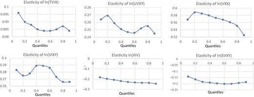
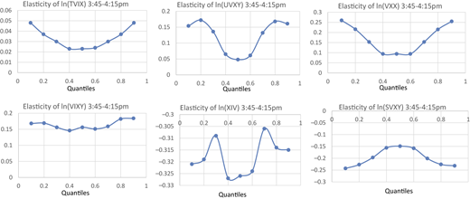
We now turn to assessing the elasticity of VIX futures to VIX ETP prices using a decile regression approach. Table 1 (the corresponding graphs: Figures 1 and 2) summarizes the results of a decile regression of ln(SPVXSTR) on various ln(ETP) returns, based on the full sample of intraday 15-min log returns, excluding overnight returns. Panel A covers November 29, 2010, to February 15, 2018—when all ETNs (TVIX, VXX, XIV) traded concurrently—regressing the futures index return, ln(SPVXSTR), on ln(TVIX), ln(VXX), and ln(XIV). The coefficients, though small economically, are statistically significant at the 1% level across all deciles, confirmed by the Wald test (chi-square distribution, one degree of freedom). The constant, such as 0.096 in the first row of Panel A, indicates an SPVXSTR level of exp(0.096) or 1.10 when TVIX = VXX = XIV = 1. Panel B spans October 3, 2011, to February 15, 2018—when all ETFs (UVXY, VIXY, SVXY) traded concurrently—using all intraday data and the final 30 min before close. Elasticity, interpreted from the log coefficients, varies notably: in Panel A’s first decile, a 1% VXX return yields a 0.568% SPVXSTR return, while the reverse effect of ln(SPVXSTR) on ln(VXX) is 1/0.568 or 1.761%, enabled by cointegration of all variables. Updated results reveal elasticity is lower at the close but higher intraday, possibly due to liquidity differences, and peaks at the distribution’s extreme ends at close. For example, a 1% change in VXX corresponds to an 0.568% change in SPVXSTR during intraday trading and a 0.260% change at market close at the first decile. Similarly, a 1% change in VIXY corresponds to an 0.283% change in SPVXSTR during intraday trading and a 0.168% change at market close at the first decile. Comparing ETNs and ETFs, XIV and SVXY show similar elasticity, while TVIX’s elasticity is half that of UVXY, consistent with TVIX’s leverage ratio being halved. Notably, VXX exhibits much higher elasticity than VIXY, likely due to its dominance as an unhedged note structure, unlike ETFs. Sensitivity of SPVXSTR to XIV increases across Panel A’s higher deciles intraday, though it diminishes at close, reflecting shifting hedging demands.

The research findings carry significant implications for understanding VIX futures and ETP dynamics. The observation that elasticity is lower at market close but higher during the trading day, potentially due to liquidity differences, suggests that intraday trading conditions amplify the responsiveness of VIX futures to ETP price changes, offering traders opportunities to exploit these variations (O’Neill and Rajaguru, 2024). The heightened elasticity at the extreme ends of the distribution at close implies that during volatile closing periods, VIX futures may overreact to ETP movements, impacting hedging strategies in stress scenarios. The similar elasticity between XIV ETNs and SVXY ETFs indicates that structural differences between ETNs and ETFs may not significantly alter their influence on VIX futures, providing flexibility in instrument choice for investors. In contrast, the finding that TVIX ETNs exhibit half the elasticity of UVXY ETFs, aligning with TVIX’s reduced leverage ratio, underscores how leverage adjustments directly shape market impact. Finally, the notably higher elasticity of VXX compared to VIXY ETFs, likely due to VXX’s dominance and unhedged note structure, highlights its outsized role in driving VIX futures, relative to ETF counterparts, with implications for portfolio construction and volatility trading (O’Neill and Rajaguru, 2023).

This paper examines the elasticity dynamics between VIX ETPs and VIX Futures contracts. VIX product markets have expanded to rival SPX and SPY options as leading platforms for trading and hedging volatility. This surge in investor activity has been accompanied by evolving causal relationships between VIX Futures and ETPs over time.

Decile regressions highlight the sensitivity of VIX Futures prices to ETP prices and how these changes in different volatility environments. Results show that VIX futures, as proxied by SPVXSTR, are more responsive to VXX, than to TVIX and XIV except 3:45–4:15p.m. where XIV is dominant. Results also show increasing sensitivity of SPVXSTR to XIV across the full day (panel A) in higher deciles, where higher returns on VIX futures may well drive higher hedging demands for such products such that hedging is brought-forward earlier in the day. Similarly, the results for the associated ETFs, which are less actively traded, are more ambiguous. Practically speaking, the higher elasticity during the trading day means that intraday trading conditions amplify the responsiveness of VIX futures to ETP price changes. Traders may seek to exploit these variations. Similarly, elasticity is heightened at the extreme ends of the distribution at close. VIX futures may overreact to ETP movements and this has implications for calibrating hedging strategies in stress scenarios.
Agapova
,
A.
(
2011
), “
Conventional mutual index funds versus exchange-traded funds
”,
Journal of Financial Markets
, Vol. 
14
No. 
2
, pp. 
323
-
343
, doi: .
Alexander
,
C.
and
Korovilas
,
D.
(
2013
), “
Volatility exchange-traded notes: curse or cure?
”,
The Journal of Alternative Investments
, Vol. 
16
No. 
2
, pp. 
52
-
70
, doi: .
Benos
,
E.
and
Sagade
,
S.
(
2016
), “
Price discovery and the cross-section of high-frequency trading
”,
Journal of Financial Markets
, Vol. 
30
, pp. 
54
-
77
, doi: .
Bollen
,
N.P.B.
,
O'Neill
,
M.J.
and
Whaley
,
R.E.
(
2017
), “
Tail wags dog: intraday price discovery in VIX markets
”,
Journal of Futures Markets
, Vol. 
37
No. 
5
, pp. 
431
-
451
, doi: .
Bordonado
,
C.
,
Moln´ar
,
P.
and
Samdal
,
S.R.
(
2017
), “
VIX exchange traded products: price discovery, hedging, and trading strategy
”,
Journal of Futures Markets
, Vol. 
37
No. 
2
, pp. 
164
-
183
, doi: .
Broman
,
M.S.
(
2016
), “
Liquidity, style investing and excess comovement of exchange-traded fund returns
”,
Journal of Financial Markets
, Vol. 
30
 
C
, pp.
27
-
53
.
Fernandez-Perez
,
A.
,
Frijns
,
B.
,
Gafiatullina
,
I.
and
Tourani-Raid
,
A.
(
2018
), “
Determinants of intraday price discovery in VIX exchange traded notes
”,
Journal of Futures Markets
, Vol. 
38
No. 
5
, pp. 
535
-
548
, doi: .
Fleming
,
J.
,
Ostdiek
,
B.
and
Whaley
,
R.E.
(
1996
), “
Trading costs and the relative rates of price discovery in stock, futures, and option markets
”,
Journal of Futures Markets
, Vol. 
16
No. 
4
, pp. 
353
-
387
, doi: .
Frijns
,
B.
,
Tourani-Rad
,
A.
and
Webb
,
R.I.
(
2016
), “
On the intraday relation between the VIX and its futures
”,
Journal of Futures Markets
, Vol. 
36
No. 
9
, pp. 
870
-
886
, doi: .
Gehricke
,
S.
and
Zhang
,
J.
(
2018
), “
Modelling VVX
”,
Journal of Futures Markets
, Vol. 
38
No. 
8
, pp. 
958
-
976
, doi: .
Hill
,
J.
(
2013
), “
The different faces of volatility exposure in portfolio management
”,
The Journal of Alternative Investments
, Vol. 
15
No. 
3
, pp. 
9
-
31
, doi: .
Johnson
,
T.L.
(
2017
), “
Risk premium and the VIX term structure
”,
Journal of Financial and Quantitative Analysis
, Vol. 
52
No. 
6
, pp. 
2461
-
2490
, doi: .
Koenker
,
R.
(
2005
),
Quantile Regressions
, (1st ed.) ,
Cambridge University Press
,
New York
.
Koenker
,
R.
and
Hallock
,
K.
(
2001
), “
Quantile regression
”,
Journal of Economic Perspectives
, Vol. 
15
, pp. 
143
-
156
.
Lin
,
Y.N.
(
2007
), “
Pricing VIX futures: evidence from integrated physical and risk neutral probability measures
”,
Journal of Futures Markets
, Vol. 
27
No. 
12
, pp. 
1175
-
1217
, doi: .
O'Neill
,
M.
and
Rajaguru
,
G.
(
2019
), “
A response surface analysis of critical values for the lead-lag ratio with application to high frequency and non-synchronous financial data
”,
Accounting and Finance
, Vol. 
60
No. 
4
, pp. 
3979
-
3990
, doi: .
O'Neill
,
M.
and
Rajaguru
,
G.
(
2023
), “
Causality of price movements in VIX exchange-traded products and VIX futures contracts
”,
Journal of Accounting Literature
, Vol. 
46
No. 
2
, pp. 
1
-
17
.
O'Neill
,
M.
and
Rajaguru
,
G.
(
2024
), “
On the analysis of time varying causality between VIX Exchange-Traded Products and VIX Futures Contracts in high and low volatility regimes
”,
Journal of Accounting Literature
, Vol. 
47
No. 
5
, pp. 
99
-
109
, doi: .
O'Neill
,
M.J.
and
Whaley
,
R.E.
(
2023
), “
Effects of nondiscretionary trading on futures prices
”,
Journal of Futures Markets
, Vol. 
43
No. 
1
, pp. 
33
-
68
, doi: .
Ozturk
,
S.R.
,
van der Wel
,
M.
and
van Dijk
,
D.
(
2017
), “
Intraday price discovery in fragmented markets
”,
Journal of Financial Markets
, Vol. 
32
, pp. 
28
-
48
, doi: .
Park
,
Y.H.
(
2015
), “
Volatility-of-volatility and tail risk hedging returns
”,
Journal of Financial Markets
, Vol. 
26
, pp. 
38
-
63
, doi: .
Posselt
,
A.M.
(
2021
), “
Dynamics in the VIX complex
”,
Journal of Futures Markets
, Vol. 
42
No. 
9
, pp. 
1
-
23
, doi: .
Riordan
,
R.
and
Storkenmaier
,
A.
(
2012
), “
Latency, liquidity and price discovery
”,
Journal of Financial Markets
, Vol. 
15
No. 
4
, pp. 
416
-
437
, doi: .
Shu
,
J.
and
Zhang
,
J.
(
2012
), “
Causality in the VIX futures market
”,
Journal of Futures Markets
, Vol. 
32
No. 
1
, pp. 
24
-
46
, doi: .
Whaley
,
R.E.
(
1993
), “
Derivatives on market volatility: hedging tools long overdue
”,
Journal of Derivatives
, Vol. 
1
, pp. 
71
-
84
, doi: .
Whaley
,
R.E.
(
2013
), “
Volatility trading: at what cost?
”,
Journal of Portfolio Management
, Vol. 
40
No. 
1
, pp. 
95
-
108
, doi: .
Zhu
,
S.P.
and
Lian
,
G.H.
(
2012
), “
An analytical formula for VIX futures and its applications
”,
Journal of Futures Markets
, Vol. 
32
No. 
2
, pp. 
166
-
190
, doi: .
Published by Emerald Publishing Limited. This article is published under the Creative Commons Attribution (CC BY 4.0) licence. Anyone may reproduce, distribute, translate and create derivative works of this article (for both commercial and non-commercial purposes), subject to full attribution to the original publication and authors. The full terms of this licence may be seen at Link to the terms of the CC BY 4.0 licence.

Data & Figures

Figure 1
Six line graphs show the elasticity of different variables against quantiles.In all six graphs, the horizontal axis is labeled “Quantiles” and has markings ranging from 0 to 1 in increments of 0.2 units. Graph 1: The graph is titled “Elasticity of T V I X”. The vertical axis has markings ranging from 0.08 to 0.1 in increments of 0.005 units. The graph shows a line that starts from (0.1, 0.096), moves downward passing through (0.2, 0.09), (0.4, 0.085), (0.6, 0.084), rises again to (0.8, 0.087), and terminates at (0.9, 0.084). Graph 2: The graph is titled “Elasticity of U V X Y”. The vertical axis has markings ranging from 0.24 to 0.28 in increments of 0.01 units. The graph shows a line that starts from (0.1, 0.263), rises upward to (0.2, 0.269), slopes down passing through (0.3, 0.258), (0.6, 0.245), rises again to (0.8, 0.255), and terminates at (0.9, 0.244). Graph 3: The graph is titled “Elasticity of V X X”. The vertical axis has markings ranging from 0.52 to 0.6 in increments of 0.02 units. The graph shows a line that starts from (0.1, 0.566), rises upward to (0.2, 0.589), slopes downward passing through (0.4, 0.58), (0.7, 0.56), and terminates at (0.9, 0.524). Graph 4: The graph is titled “Elasticity of V I X Y”. The vertical axis has markings ranging from 0.26 to 0.3 in increments of 0.01 units. The graph shows a line that starts from (0.1, 0.283), slopes down to (0.2, 0.275), rises upward to (0.4, 0.289), slopes down again passing through (0.6, 0.286), (0.7, 0.273), (0.8, 0.266), and terminates at (0.9, 0.267). Graph 5: The graph is titled “Elasticity of X I V”. The vertical axis has markings ranging from negative 0.3 to 0 in increments of 0.1 units. The graph shows a line that starts from (0.1, negative 0.18), slopes downward, passing through (0.3, negative 0.21), (0.5, negative 0.23), (0.7, negative 0.24), and terminates at (0.9, negative 0.25). Graph 6: The graph is titled “Elasticity of S V X Y”. The vertical axis has markings ranging from negative 0.25 to 0 in increments of 0.05 units. The graph shows a line that starts from (0.1, negative 0.14), slopes downward passing through (0.2, negative 0.16), (0.39, negative 0.19), (0.6, negative 0.2), (0.8, negative 0.19), and terminates at (0.9, negative 0.18). Note: All numerical data values are approximated.

Full sample results: elasticities at different quantiles, dependent variable: ln(SPVXSTER). Note(s): Figure shows the elasticities of a decile regression fitted with the dependent variable being ln(SPVXSTR) and the independent variables natural logarithm of 15-min ETP returns. The regression is fitted over the entire period. Source(s): Authors’ own work

Figure 1
Six line graphs show the elasticity of different variables against quantiles.In all six graphs, the horizontal axis is labeled “Quantiles” and has markings ranging from 0 to 1 in increments of 0.2 units. Graph 1: The graph is titled “Elasticity of T V I X”. The vertical axis has markings ranging from 0.08 to 0.1 in increments of 0.005 units. The graph shows a line that starts from (0.1, 0.096), moves downward passing through (0.2, 0.09), (0.4, 0.085), (0.6, 0.084), rises again to (0.8, 0.087), and terminates at (0.9, 0.084). Graph 2: The graph is titled “Elasticity of U V X Y”. The vertical axis has markings ranging from 0.24 to 0.28 in increments of 0.01 units. The graph shows a line that starts from (0.1, 0.263), rises upward to (0.2, 0.269), slopes down passing through (0.3, 0.258), (0.6, 0.245), rises again to (0.8, 0.255), and terminates at (0.9, 0.244). Graph 3: The graph is titled “Elasticity of V X X”. The vertical axis has markings ranging from 0.52 to 0.6 in increments of 0.02 units. The graph shows a line that starts from (0.1, 0.566), rises upward to (0.2, 0.589), slopes downward passing through (0.4, 0.58), (0.7, 0.56), and terminates at (0.9, 0.524). Graph 4: The graph is titled “Elasticity of V I X Y”. The vertical axis has markings ranging from 0.26 to 0.3 in increments of 0.01 units. The graph shows a line that starts from (0.1, 0.283), slopes down to (0.2, 0.275), rises upward to (0.4, 0.289), slopes down again passing through (0.6, 0.286), (0.7, 0.273), (0.8, 0.266), and terminates at (0.9, 0.267). Graph 5: The graph is titled “Elasticity of X I V”. The vertical axis has markings ranging from negative 0.3 to 0 in increments of 0.1 units. The graph shows a line that starts from (0.1, negative 0.18), slopes downward, passing through (0.3, negative 0.21), (0.5, negative 0.23), (0.7, negative 0.24), and terminates at (0.9, negative 0.25). Graph 6: The graph is titled “Elasticity of S V X Y”. The vertical axis has markings ranging from negative 0.25 to 0 in increments of 0.05 units. The graph shows a line that starts from (0.1, negative 0.14), slopes downward passing through (0.2, negative 0.16), (0.39, negative 0.19), (0.6, negative 0.2), (0.8, negative 0.19), and terminates at (0.9, negative 0.18). Note: All numerical data values are approximated.

Full sample results: elasticities at different quantiles, dependent variable: ln(SPVXSTER). Note(s): Figure shows the elasticities of a decile regression fitted with the dependent variable being ln(SPVXSTR) and the independent variables natural logarithm of 15-min ETP returns. The regression is fitted over the entire period. Source(s): Authors’ own work

Close modal
Figure 2
Six line graphs display elasticity curves across quantiles during the 3:45 to 4:15 p m period”.In all six graphs, the horizontal axis is labeled “Quantiles” and has markings ranging from 0 to 1 in increments of 0.2 units. Graph 1: The graph is titled “Elasticity of T V I X 3:45 to 4:15 p m”. The vertical axis has markings ranging from 0.01 to 0.06 in increments of 0.01 units. The graph shows a concave up curve that starts from (0.1, 0.049), slopes down to (0.5, 0.22), rises upward, and terminates at (0.9, 0.049). Graph 2: The graph is titled “Elasticity of U V X Y 3:45 to 4:15 p m”. The vertical axis has markings ranging from 0 to 0.2 in increments of 0.05 units. The graph shows a curve that starts from (0.1, 0.16), rises upward to (0.2, 0.17), slopes down passing through (0.3, 0.14), (0.5, 0.05), rises upward to (0.8, 0.17), and terminates at (0.9, 0.16). Graph 3: The graph is titled “Elasticity of V X X 3:45 to 4:15 p m”. The vertical axis has markings ranging from 0 to 0.3 in increments of 0.05 units. The graph shows a concave up curve that starts from (0.1, 0.26), slopes down to (0.4, 0.09), (0.5, 0.09), (0.6, 0.1), rises upward to (0.8, 0.21), and terminates at (0.9, 0.26). Graph 4: The graph is titled “Elasticity of V I X Y 3:45 to 4:15 p m”. The vertical axis has markings ranging from 0 to 0.2 in increments of 0.05 units. The graph shows a curve that starts from (0.1, 0.17), moves to the right passing through coordinates (0.2, 0.17), (0.3, 0.16), (0.4, 0.15), (0.5, 0.16), (0.6, 0.15), (0.7, 0.16), (0.8, 0.18), and terminates at (0.9, 0.19). Graph 5: The graph is titled “Elasticity of X I V 3:45 to 4:15 p m”. The vertical axis has markings ranging from negative 0.33 to negative 0.3 in increments of 0.005 units. The graph shows a curve that starts from (0.1, negative 0.321), rises upward passing through (0.2, negative 0.32), (0.3, negative 0.31), slopes down to (0.4, negative 0.327), rises upward again passing through coordinates (0.6, negative 0.325), (0.7, negative 0.306), and terminates at (0.9, negative 0.315). Graph 6: The graph is titled “Elasticity of S V X Y 3:45 to 4:15 p m”. The vertical axis has markings ranging from negative 0.3 to 0 in increments of 0.05 units. The graph shows a concave down curve that starts from (0.1, negative 0.24), rises upward passing through (0.3, negative 0.2), (0.5, negative 0.15), slopes downward to (0.7, negative 0.2), and terminates at (0.9, negative 0.23). Note: All numerical data values are approximated.

Closing sample results: elasticities at different quantiles, dependent variable: SPVXSTER. Note(s): Figure shows the elasticities of a decile regression fitted with the dependent variable being ln(SPVXSTR) and the independent variables natural logarithm of 15-min ETP returns. The regression is fitted over the closing sample. Source(s): Authors’ own work

Figure 2
Six line graphs display elasticity curves across quantiles during the 3:45 to 4:15 p m period”.In all six graphs, the horizontal axis is labeled “Quantiles” and has markings ranging from 0 to 1 in increments of 0.2 units. Graph 1: The graph is titled “Elasticity of T V I X 3:45 to 4:15 p m”. The vertical axis has markings ranging from 0.01 to 0.06 in increments of 0.01 units. The graph shows a concave up curve that starts from (0.1, 0.049), slopes down to (0.5, 0.22), rises upward, and terminates at (0.9, 0.049). Graph 2: The graph is titled “Elasticity of U V X Y 3:45 to 4:15 p m”. The vertical axis has markings ranging from 0 to 0.2 in increments of 0.05 units. The graph shows a curve that starts from (0.1, 0.16), rises upward to (0.2, 0.17), slopes down passing through (0.3, 0.14), (0.5, 0.05), rises upward to (0.8, 0.17), and terminates at (0.9, 0.16). Graph 3: The graph is titled “Elasticity of V X X 3:45 to 4:15 p m”. The vertical axis has markings ranging from 0 to 0.3 in increments of 0.05 units. The graph shows a concave up curve that starts from (0.1, 0.26), slopes down to (0.4, 0.09), (0.5, 0.09), (0.6, 0.1), rises upward to (0.8, 0.21), and terminates at (0.9, 0.26). Graph 4: The graph is titled “Elasticity of V I X Y 3:45 to 4:15 p m”. The vertical axis has markings ranging from 0 to 0.2 in increments of 0.05 units. The graph shows a curve that starts from (0.1, 0.17), moves to the right passing through coordinates (0.2, 0.17), (0.3, 0.16), (0.4, 0.15), (0.5, 0.16), (0.6, 0.15), (0.7, 0.16), (0.8, 0.18), and terminates at (0.9, 0.19). Graph 5: The graph is titled “Elasticity of X I V 3:45 to 4:15 p m”. The vertical axis has markings ranging from negative 0.33 to negative 0.3 in increments of 0.005 units. The graph shows a curve that starts from (0.1, negative 0.321), rises upward passing through (0.2, negative 0.32), (0.3, negative 0.31), slopes down to (0.4, negative 0.327), rises upward again passing through coordinates (0.6, negative 0.325), (0.7, negative 0.306), and terminates at (0.9, negative 0.315). Graph 6: The graph is titled “Elasticity of S V X Y 3:45 to 4:15 p m”. The vertical axis has markings ranging from negative 0.3 to 0 in increments of 0.05 units. The graph shows a concave down curve that starts from (0.1, negative 0.24), rises upward passing through (0.3, negative 0.2), (0.5, negative 0.15), slopes downward to (0.7, negative 0.2), and terminates at (0.9, negative 0.23). Note: All numerical data values are approximated.

Closing sample results: elasticities at different quantiles, dependent variable: SPVXSTER. Note(s): Figure shows the elasticities of a decile regression fitted with the dependent variable being ln(SPVXSTR) and the independent variables natural logarithm of 15-min ETP returns. The regression is fitted over the closing sample. Source(s): Authors’ own work

Close modal
Table 1

Decile regression of VIX futures on VIX ETPs for the period November 29, 2010 through February 15, 2018

Panel A - VXX, TVIX and XIV ETNs with SPVXSTER
Full sample3:45–4:15p.m.
Decileln(TVIX)ln(VXX)ln(XIV)ConstantDecileln(TVIX)ln(VXX)ln(XIV)Constant
0.10.0960.568−0.1830.0960.10.0480.260−0.321−0.0004
0.20.0900.588−0.1970.0900.20.0370.216−0.319−0.0002
0.30.0880.585−0.2070.0880.30.0300.153−0.309−0.00008
0.40.0850.580−0.2190.0850.40.0230.094−0.327−0.00003
0.50.0840.573−0.2280.0840.50.0230.094−0.3260.0000
0.60.0840.568−0.2330.0840.60.0240.094−0.3240.00007
0.70.0850.561−0.2360.0850.70.0300.153−0.3060.00008
0.80.0870.551−0.2370.0870.80.0370.215−0.3140.0002
0.90.0840.525−0.2450.0840.90.0480.255−0.3150.0004
Panel B - VIXY, UVXY and SVXY ETFs with SPVXSTER
Full sample3:45–4:15p.m.
Decileln(UVXY)ln(VIXY)ln(SVXY)ConstantDecileln(UVXY)ln(VIXY)ln(SVXY)Constant
0.10.2640.283−0.1420.2640.10.1540.168−0.243−0.001
0.20.2690.275−0.1650.2690.20.1720.169−0.227−0.0007
0.30.2590.278−0.1850.2590.30.1360.156−0.197−0.0003
0.40.2510.289−0.1910.2510.40.0650.146−0.156−0.00004
0.50.2470.289−0.1980.2470.50.0480.156−0.1490.00000
0.60.2460.286−0.2020.2460.60.0610.151−0.1580.00004
0.70.2520.273−0.2010.2520.70.1320.159−0.2010.0003
0.80.2550.266−0.1940.2550.80.1680.182−0.2260.0007
0.90.2450.266−0.1870.2450.90.1610.184−0.2320.001

Note(s): Table shows the coefficients of a decile regression fitted with the dependent variable being ln(SPVXSTR) and the independent variables natural logarithm of 15 min ETP returns. The regression is fitted over the entire period. Panel A contains the results using November 29, 2010 through February 15, 2018—the period during which all ETNs were traded concurrently. Panel B contains the results using October 3, 2011 through February 15, 2018—the period during which all ETFs were traded concurrently. All estimated coefficients are significant at the one percent probability level

Source(s): Authors’ own work

Supplements

References

Agapova
,
A.
(
2011
), “
Conventional mutual index funds versus exchange-traded funds
”,
Journal of Financial Markets
, Vol. 
14
No. 
2
, pp. 
323
-
343
, doi: .
Alexander
,
C.
and
Korovilas
,
D.
(
2013
), “
Volatility exchange-traded notes: curse or cure?
”,
The Journal of Alternative Investments
, Vol. 
16
No. 
2
, pp. 
52
-
70
, doi: .
Benos
,
E.
and
Sagade
,
S.
(
2016
), “
Price discovery and the cross-section of high-frequency trading
”,
Journal of Financial Markets
, Vol. 
30
, pp. 
54
-
77
, doi: .
Bollen
,
N.P.B.
,
O'Neill
,
M.J.
and
Whaley
,
R.E.
(
2017
), “
Tail wags dog: intraday price discovery in VIX markets
”,
Journal of Futures Markets
, Vol. 
37
No. 
5
, pp. 
431
-
451
, doi: .
Bordonado
,
C.
,
Moln´ar
,
P.
and
Samdal
,
S.R.
(
2017
), “
VIX exchange traded products: price discovery, hedging, and trading strategy
”,
Journal of Futures Markets
, Vol. 
37
No. 
2
, pp. 
164
-
183
, doi: .
Broman
,
M.S.
(
2016
), “
Liquidity, style investing and excess comovement of exchange-traded fund returns
”,
Journal of Financial Markets
, Vol. 
30
 
C
, pp.
27
-
53
.
Fernandez-Perez
,
A.
,
Frijns
,
B.
,
Gafiatullina
,
I.
and
Tourani-Raid
,
A.
(
2018
), “
Determinants of intraday price discovery in VIX exchange traded notes
”,
Journal of Futures Markets
, Vol. 
38
No. 
5
, pp. 
535
-
548
, doi: .
Fleming
,
J.
,
Ostdiek
,
B.
and
Whaley
,
R.E.
(
1996
), “
Trading costs and the relative rates of price discovery in stock, futures, and option markets
”,
Journal of Futures Markets
, Vol. 
16
No. 
4
, pp. 
353
-
387
, doi: .
Frijns
,
B.
,
Tourani-Rad
,
A.
and
Webb
,
R.I.
(
2016
), “
On the intraday relation between the VIX and its futures
”,
Journal of Futures Markets
, Vol. 
36
No. 
9
, pp. 
870
-
886
, doi: .
Gehricke
,
S.
and
Zhang
,
J.
(
2018
), “
Modelling VVX
”,
Journal of Futures Markets
, Vol. 
38
No. 
8
, pp. 
958
-
976
, doi: .
Hill
,
J.
(
2013
), “
The different faces of volatility exposure in portfolio management
”,
The Journal of Alternative Investments
, Vol. 
15
No. 
3
, pp. 
9
-
31
, doi: .
Johnson
,
T.L.
(
2017
), “
Risk premium and the VIX term structure
”,
Journal of Financial and Quantitative Analysis
, Vol. 
52
No. 
6
, pp. 
2461
-
2490
, doi: .
Koenker
,
R.
(
2005
),
Quantile Regressions
, (1st ed.) ,
Cambridge University Press
,
New York
.
Koenker
,
R.
and
Hallock
,
K.
(
2001
), “
Quantile regression
”,
Journal of Economic Perspectives
, Vol. 
15
, pp. 
143
-
156
.
Lin
,
Y.N.
(
2007
), “
Pricing VIX futures: evidence from integrated physical and risk neutral probability measures
”,
Journal of Futures Markets
, Vol. 
27
No. 
12
, pp. 
1175
-
1217
, doi: .
O'Neill
,
M.
and
Rajaguru
,
G.
(
2019
), “
A response surface analysis of critical values for the lead-lag ratio with application to high frequency and non-synchronous financial data
”,
Accounting and Finance
, Vol. 
60
No. 
4
, pp. 
3979
-
3990
, doi: .
O'Neill
,
M.
and
Rajaguru
,
G.
(
2023
), “
Causality of price movements in VIX exchange-traded products and VIX futures contracts
”,
Journal of Accounting Literature
, Vol. 
46
No. 
2
, pp. 
1
-
17
.
O'Neill
,
M.
and
Rajaguru
,
G.
(
2024
), “
On the analysis of time varying causality between VIX Exchange-Traded Products and VIX Futures Contracts in high and low volatility regimes
”,
Journal of Accounting Literature
, Vol. 
47
No. 
5
, pp. 
99
-
109
, doi: .
O'Neill
,
M.J.
and
Whaley
,
R.E.
(
2023
), “
Effects of nondiscretionary trading on futures prices
”,
Journal of Futures Markets
, Vol. 
43
No. 
1
, pp. 
33
-
68
, doi: .
Ozturk
,
S.R.
,
van der Wel
,
M.
and
van Dijk
,
D.
(
2017
), “
Intraday price discovery in fragmented markets
”,
Journal of Financial Markets
, Vol. 
32
, pp. 
28
-
48
, doi: .
Park
,
Y.H.
(
2015
), “
Volatility-of-volatility and tail risk hedging returns
”,
Journal of Financial Markets
, Vol. 
26
, pp. 
38
-
63
, doi: .
Posselt
,
A.M.
(
2021
), “
Dynamics in the VIX complex
”,
Journal of Futures Markets
, Vol. 
42
No. 
9
, pp. 
1
-
23
, doi: .
Riordan
,
R.
and
Storkenmaier
,
A.
(
2012
), “
Latency, liquidity and price discovery
”,
Journal of Financial Markets
, Vol. 
15
No. 
4
, pp. 
416
-
437
, doi: .
Shu
,
J.
and
Zhang
,
J.
(
2012
), “
Causality in the VIX futures market
”,
Journal of Futures Markets
, Vol. 
32
No. 
1
, pp. 
24
-
46
, doi: .
Whaley
,
R.E.
(
1993
), “
Derivatives on market volatility: hedging tools long overdue
”,
Journal of Derivatives
, Vol. 
1
, pp. 
71
-
84
, doi: .
Whaley
,
R.E.
(
2013
), “
Volatility trading: at what cost?
”,
Journal of Portfolio Management
, Vol. 
40
No. 
1
, pp. 
95
-
108
, doi: .
Zhu
,
S.P.
and
Lian
,
G.H.
(
2012
), “
An analytical formula for VIX futures and its applications
”,
Journal of Futures Markets
, Vol. 
32
No. 
2
, pp. 
166
-
190
, doi: .

Languages

or Create an Account

Close Modal
Close Modal
