The impact of uncertainty, financial market dynamics and commodity indices on green asset price forecastability: evidence from advanced data-driven methods

In recent years, green finance has gained significant attention as climate change and environmental protection have emerged as global priorities. Financial markets have responded by developing a mixture of green financial assets, including, among others, green bonds and renewable energy stocks (Pham et al., 2024). In addition, legislative frameworks and international agreements have been established to promote transparency, standardization and accountability in green finance, thereby strengthening investor confidence and facilitating greater capital mobilization for sustainable projects (Mohamad, 2025). Consequently, green investments have garnered considerable interest from investors across both bond and equity markets (Pham et al., 2024).

As green finance has taken on increasing importance in financial markets, the literature on green stocks has expanded rapidly and now falls into three main strands. The first strand examines the financial performance, risk characteristics and diversification benefits of green assets (Pham, 2016; Reboredo, 2018; Broadstock et al., 2021). The second strand explores the hedging and safe-haven properties of green assets against traditional assets and uncertainty shocks (Reboredo and Ugolini, 2020; Umar et al., 2022). The third and more recent strand investigates the dynamic interconnections between green assets and traditional financial and energy markets, highlighting the importance of spillover and predictive relationships (Chatziantoniou et al., 2022; Kocaarslan and Soytas, 2023; Ben Amor et al., 2026).

This study addresses a research gap within the third area of literature on green assets. While earlier research has focused on a single segment of green assets, mainly green bonds, other sectors, such as clean energy and water markets, have received limited interest. Furthermore, many analyses rely on traditional linear econometric models, which may fail to capture the nonlinear and dynamic behavior of green asset prices. In addition, the influence of global macroeconomic factors and commodity price movements on the performance of green assets remains insufficiently explored in the literature, revealing a lack of comprehensive analysis. Finally, only a few studies clearly identify the most significant predictors in forecasting models, which limits their practical usefulness for investors and policymakers. Therefore, adopting advanced data-driven approaches, such as machine and deep learning models, appears essential for forecasting green assets.

In this context, our study aims to extend current research by providing a predictive analysis of four major indices (the S&P Green Bond Index, the S&P Global Clean Energy Index, the S&P GSCI Water Index and the MSCI Global Environment Index) based on daily observations collected between January 2018 and December 2024. The objective is to forecast their prices and to identify the key factors influencing their performance. For this reason, other variables such as the MSCI World Index, the VIX, the S&P U.S. Aggregate Bond Index and several commodity indices have been used as influencing factors and their predictive power is determined using the SHAP approach. For the methodology, we compare machine learning algorithms, mainly Random Forest (RF), Extreme Gradient Boosting (XGBoost) and Light Gradient Boosting Machine (LightGBM), with deep learning architectures, specifically Recurrent Neural Network (RNN), Long Short-Term Memory (LSTM) and Gated Recurrent Unit (GRU). We assess their performance using four metrics: the coefficient of determination (R²), the mean absolute error (MAE), the mean squared error (MSE) and the root mean square error (RMSE).

The contribution of this study is in four parts. First, although existing studies have explored the interactions between green assets and conventional financial markets, these dynamics remain only partially understood, particularly given the diversity of green sectors. This study extends the analysis by investigating four green market indices. We integrate a diverse set of financial and commodity variables, including the MSCI World Index, VIX, S&P U.S. Aggregate Bond Index and major commodities such as Gold, Silver, Crude Oil and Gas Oil. This approach provides an understanding of the green market's sensitivity to global financial dynamics. To the best of our knowledge, this is among the first studies to jointly examine four distinct green financial indices within a unified comparative framework. Second, we apply the SHAP approach during the training phase. This method decomposes feature contributions, showing which financial or commodity factors influence green asset performance across models and indices. Our comparative analysis reveals substantial heterogeneity in the sensitivity of green indices to financial and commodity markets. While the green bond (SPGBI) and clean energy (SGCEI) indices exhibit clear and significant negative relationships with energy prices, the water (SGWI) and environmental (MSCI.ENV) indices show largely ambiguous relationships with these same variables, challenging the assumption of a homogeneous “green finance” segment. Third, we use machine and deep learning techniques to evaluate and compare forecasting performance in modeling the nonlinear behavior of green assets. Out-of-sample evaluations using R², MAE, MSE and RMSE metrics identify the most effective model for each green index. Fourth, this study provides guidance for investors and policymakers by analyzing what determines the performance of different segments within the green finance market. The results can support investment decisions and the development of sustainability-focused financial policies.

The main results of this paper indicate that conventional and developed markets continue to shape green asset dynamics, as revealed by the SHAP analysis. Among the predictive models evaluated, deep learning models generally provide high accuracy. Specifically, the GRU technique outperforms other models for green bonds and the water index. Predictions from the GRU model closely match actual values, confirming the model's predictive capacity. The findings highlight major factors, such as the S&P U.S. Aggregate Bond Index and the MSCI World Index, as significant drivers for almost all green assets.

The remainder of this study presents the following structure. Section 2 reviews the literature. Section 3 presents the methodology. Section 4 reports and interprets the results. Section 5 concludes and discusses the implications for research and policy.

The forecasting of green assets, including green bonds and environmentally stock indices, has attracted growing attention from policymakers and academics due to the increasing importance of climate risk and sustainable investment.

Several studies have addressed modeling approaches for risk and return prediction. For instance, Liu (2022) shows that traditional fixed-income, equity, currency and energy markets collectively drive green bond volatility, highlighting the need to consider multiple markets when predicting green asset risks. Xia et al. (2022) develop ensemble tree-based models combining financial and commodity predictors to forecast green bond volatility. Adekoya et al. (2023) confirm that financial and commodity variables significantly influence green bond returns, with asymmetric models outperforming symmetric ones. Zhuo et al. (2023) identify GARCH and GARCH-FZ models as the most effective for extreme risk forecasting in green bond and clean energy markets.

Recently, machine learning and deep learning methods have been increasingly applied to green bond forecasting. Çetin (2022) predicts the corporate green bond index using a neural network with conventional bond indices as inputs, achieving high accuracy. Wang et al. (2022) combine LSTM with EMD and CEEMDAN decomposition to stabilize green bond index data and improve prediction accuracy. Kocaarslan and Soytas (2023) apply Random Forest, XGBoost, CatBoost and LightGBM to assess the influence of conventional bonds, stocks and energy commodities on U.S. municipal green bond performance. Nie et al. (2023) employ LSTM with optimal exogenous variables to forecast China's green bond yields.

More recently, studies in financial forecasting have focused on hybrid and ensemble learning architectures as effective tools for capturing the nonlinear and dynamic nature of financial markets. For instance, Kayit and Ismail (2025) show that hybrid ensembles integrating Random Forest, Support Vector Machines, AdaBoost and LSTM significantly outperform separate models in stock market prediction tasks. Similarly, Fozap (2025) stipulates that hybrid deep learning architectures combining CNN and LSTM networks present more accurate long-term forecasts than conventional machine learning approaches. Bielskis and Belovas (2026) show that ensemble-based frameworks combining XGBoost and deep learning methods reach robust forecasting performance across major international stock indices.

Considering the increasing interest in predicting green assets, further investigation into this area becomes essential. Accordingly, the present research focuses on forecasting a range of green assets, in addition to green bonds, based on machine and deep learning models.

Numerous studies highlight different factors influencing green asset price dynamics. In this section, we focus on studies identifying conventional financial instruments and commodity markets as key determinants.

First, conventional financial instruments such as bonds, equities and currency rates are crucial in capturing the behavior of green assets. Wang et al. (2022) provide early evidence of this, confirming that financial market variables are key drivers of green bond performance in China, with indices related to oil and environmental stocks playing an important role in forecasts. Building on this, although alternative asset returns are most predictive for overall and high-frequency components, traditional financial assets remain relevant predictors within the forecasting framework when examining the role of traditional bond variables in China's green bond market (Nie et al., 2023). Extending these findings with a broader analytical framework, Adekoya et al. (2023) show that financial assets predict green bond returns across all market segments, with asymmetric models providing higher forecasting accuracy.

Second, commodity markets are also identified as key determinants of green asset price dynamics. Black et al. (2014) provide foundational evidence by emphasizing the value of including commodity prices in forecasting models. Building on this, Tu et al. (2020) and Xia et al. (2022) confirm that external factors from commodity sectors improve volatility forecasts, with SHAP values confirming their predictive significance. Wei et al. (2024) further show that commodities are important drivers of the green bond market, with WTI crude oil prices emerging as a particularly influential factor. Overall, these findings consistently point to commodities as a central determinant of green asset price dynamics.

Third, a final strand of literature considers both conventional financial and commodity markets concurrently. Hung (2021) provides early evidence by exploring the time-varying interdependence between green bonds and a broad set of assets, including the S&P 500, commodity indices and US Treasury bonds, finding that dependence is conditional and time-varying, though relatively low. Building on this, Kocaarslan and Soytas (2023) show that conventional bonds, stocks and energy commodities interact closely with green bonds, particularly during the COVID-19 pandemic, with key financial factors driving larger changes in green bond returns during periods of economic uncertainty. Extending these findings, Adekoya et al. (2023) confirm that both commodity and financial sector variables significantly influence green bond performance across all market segments, with asymmetric models yielding higher forecasting accuracy.

Building on these insights, this study empirically assesses the extent to which financial and commodity markets shape green asset price dynamics.

To achieve the objective of this study, we used daily data from January 2018 to December 2024. This period covers key transitions in the green market and periods of intense volatility associated with financial crises, making it particularly relevant for the analysis. The study examines four dependent variables of the green market, representing different segments: the S&P Green Bond Index (SPGBI), the S&P Global Clean Energy Index (SGCEI), the MSCI Environmental Index (MSCI.ENV) and the S&P Global Water Index (SGWI). These indices are used to capture different environmental investment segments, including bonds, clean energy, water and environmental equity markets.

According to the literature, we selected the following influencing factors: the MSCI World Index, the S&P U.S. Aggregate Bond Index, the VIX and a set of commodity indices, including the S&P GSCI Gold, S&P GSCI Silver, S&P GSCI Crude Oil and S&P GSCI Gas Oil. Table 1 summarizes the variables used in the analysis. In our study, the dependent variables correspond to $y$ and the independent variables correspond to $x$⁠. All data were collected from Data Stream, except the VIX provided directly by Investing.com.

Data preparation involves two steps: outlier removal and normalization. Outliers are identified using the Z-Score method, which measures the number of standard deviations a value deviates from the mean:

where $x$ is the data point, $μ$ the mean, and $σ$ is the standard deviation. Values with $|z|>3$ are flagged as outliers. This choice is based on the well-known “three standard deviations” principle: for a normally distributed variable, approximately 99.7% of observations fall within three standard deviations of the mean, so that any value beyond this limit can reasonably be considered abnormal (Aggarwal, 2016). Although other thresholds (such as |z|>2.5 or |z|>3.5) are used in the literature, |z|>3 remains by far the most commonly adopted criterion in financial time series analysis, as it offers a reasonable compromise between excessive data exclusion and the retention of extreme observations that could bias the results (Köse et al., 2025). Table 2 presents the number of outlier values identified in each variable using the Z-Score method. The VIX has the most outliers (25), followed by SGCEI (8), while the remaining variables have none. Consequently, we removed 33 rows from the dataset, resulting in a final sample of 1794 instead of 1827.

where $xmin$ and $xmax$ are the minimum and maximum values of the variable. This step ensures comparability across variables and facilitates model convergence during training (Djordjević et al., 2022).

Finally, we split the dataset into two parts, with 80% of the observations (1435) used for training, covering the period from 01/08/2018 to 23/08/2023 and 20% of the observations (359) used for testing, spanning from 24/08/2023 to 31/12/2024. We used the training set to train the models, while we evaluated their predictive performance on the test set.

Table 3 provides a summary of the descriptive statistics for all variables. The SPGBI shows moderate volatility (mean 97.13, SD 10.40), whereas the SGCEI and SGWI demonstrate higher variability, reflecting the sensitivity of clean energy and water-related assets to market fluctuations. The MSCI.ENV and MSCI World present moderate volatility, while commodities such as crude oil and gas oil are considerably more volatile, consistent with typical market dynamics. In contrast, the SPAGG remains stable (SD 7.13), whereas the VIX captures abrupt market movements with occasional extreme spikes (max 82.69). Overall, green and environmental assets display moderate to high variability, equities and commodities are more volatile than bonds and market stress periods increase volatility.

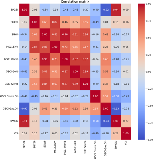
According to the correlation matrix presented in Figure 1, the SPGBI shows a positive correlation with the SPAGG (0.94). It also presents a negative correlation with the GSCI Gas.Oil (−0.92). The SGCEI shows a correlation of (0.87) with MSCI.ENV and (0.63) with the S&P Global Water Index. It also shows a positive correlation with gold (0.35). The SGWI is correlated at (0.83) with MSCI.ENV and (0.96) with the MSCI World Index. Lastly, the MSCI.ENV has a positive correlation with the MSCI World Index (0.73) and gold (0.87) and a moderate correlation with silver (0.67), highlighting its sensitivity to global market movements and safe-haven assets. These values indicate statistical associations between green indices and selected financial or commodity variables, without implying causality.

For all machine learning models presented below, the dependent variables are denoted by $y$ and the independent variables by $x$⁠.

The Random Forest (RF) algorithm, introduced by Breiman (2001), is an ensemble learning method that aggregates multiple decision trees to improve predictive performance. Each tree is trained on a bootstrap sample with a random subset of features considered at each split, reducing variance through tree decorrelation. In regression settings, the final output corresponds to the average of individual tree predictions:

where $hi(x)$ denotes the $ith$ decision tree and $x$ is the input feature vector.

The XGBoost algorithm, introduced by Chen and Guestrin (2016), is an optimized and regularized implementation of gradient boosting that uses a tree-based ensemble approach. Trees are constructed sequentially, each correcting the residual errors of the previous iteration, with predictions updated as:

Where $yˆi(t)$ and $yˆi(t−1)$ are the predictions at steps $t$ and $t−1$⁠, $xi$ is the input feature vector for observation $i$ and $ft(xi)$ is the new tree added at iteration $t$⁠.

Proposed by Ke et al. (2017), LightGBM constitutes a gradient boosting framework built upon decision tree architectures. The algorithm is characterized by a leaf-wise splitting mechanism and demonstrates strong predictive accuracy and scalability to large-scale datasets. The model consists of an ensemble of regression trees and the following describes its structure:

where $ft(x)$ refers to the tree added at iteration $t$ and $T$ is the total number of trees.

For all deep learning models presented below, the dependent variables are denoted by $y$ and the independent variables by $x$⁠.

A Recurrent Neural Network (RNN) is an artificial neural network for sequential data. RNNs incorporate a feedback mechanism whereby the hidden state at each time step is determined by both the current input and the output of the preceding step, enabling the retention of temporal dependencies across sequential data (Rizal and Soraya, 2018). For a sequence X $=(x1,x2,⋯,xT)$⁠, the hidden state $ht$ at time $t$ is:

Where $xt$​ is the input at time $t$⁠, $ht−1$ is the hidden state from the previous time step, $Wxh$ and $Whh$​ are the weight matrices, $bh$ is the bias vector and $f$ is an activation function (e.g. tanh).

Long Short-Term Memory (LSTM) networks are a type of RNN used to capture long-term dependencies in sequential data such as time series (Kuang et al., 2022). LSTM networks introduce a memory cell $Ct$ controlled by three gates: the forget gate $ft$⁠, the input gate $it$ and the output gate $οt$​, which regulate the flow of information across time steps. The cell state and hidden state are updated as:

where $☉$ denotes element-wise multiplication, $C~t$ is the candidate cell state and $ht$​ is the hidden state passed to the next time step.

The Gated Recurrent Unit (GRU), introduced by Cho et al. (2014), is a simplified variant of LSTM designed for sequential and time series data. Unlike LSTM, GRU does not include a distinct cell state, as the hidden state serves as both memory and output. The model uses two gates: the update gate $zt$⁠, which determines the portion of past information to retain and the reset gate $rt$⁠, which controls how much of the previous hidden state is disregarded when processing new input. The hidden state is updated as:

Where $ht−1$ is the previous hidden state, $zt$ is the update gate and $h~t$ is the candidate hidden state.

In this phase, the performance of the models is evaluated using four metrics, computed by comparing predicted values $yˆt$ with observed values $yt$⁠.

The MAE measures the average absolute deviation between predicted and observed values:

The MSE calculates the average of the squared differences between predicted values and observed values:

The RMSE derives from the MSE and is more sensitive to large prediction errors:

The R² measures the proportion of variance in the dependent variable explained by the model, with values closer to 1 indicating better fit:

$yˆ$⁠, $y$ and $y̅$ denote the predicted, the observed and the mean observed values, respectively.

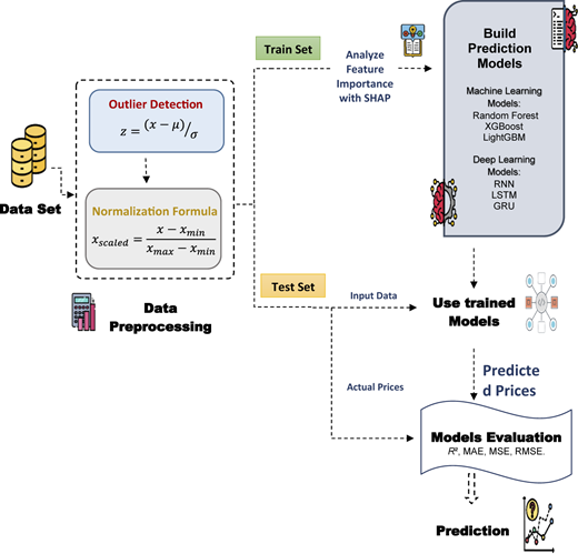
In this study, we use deep learning models (RNN, LSTM, GRU) and machine learning models (Random Forest, XGBoost, LightGBM) to forecast green market prices over the period 2018 to 2024. We detect and treat outliers using the z-score method, then normalize the data using the Min-Max method and split it into training and testing sets. We employ SHAP analysis to identify the most influential features, which we retain as explanatory variables. We evaluate model performance on the test set and through cross-validation using R², MAE, MAPE, MSE and RMSE. Figure 2 illustrates the overall methodology.

To forecast green market prices and identify the most influential variables, we employ the SHAP method (Lundberg and Lee, 2017), derived from game theory (Shapley, 1953). SHAP quantifies the contribution of each input variable to the predicted output and the variables with the strongest effect on the target are selected as inputs for model training.

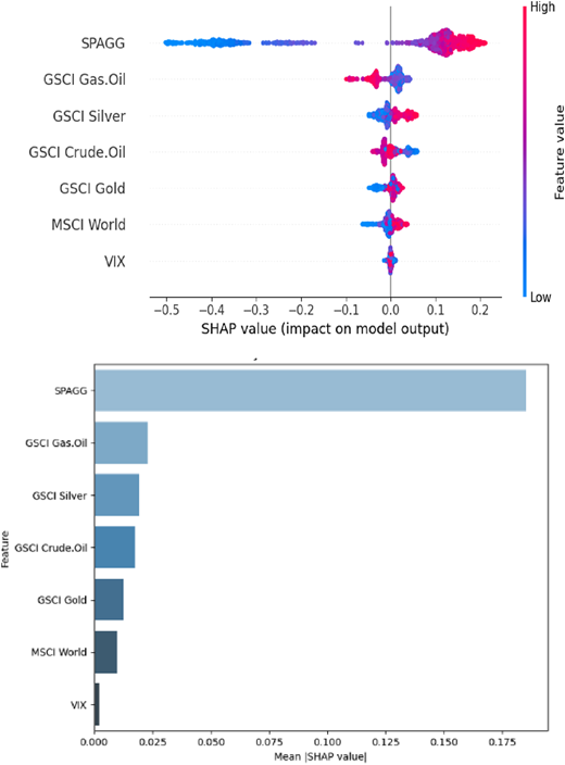
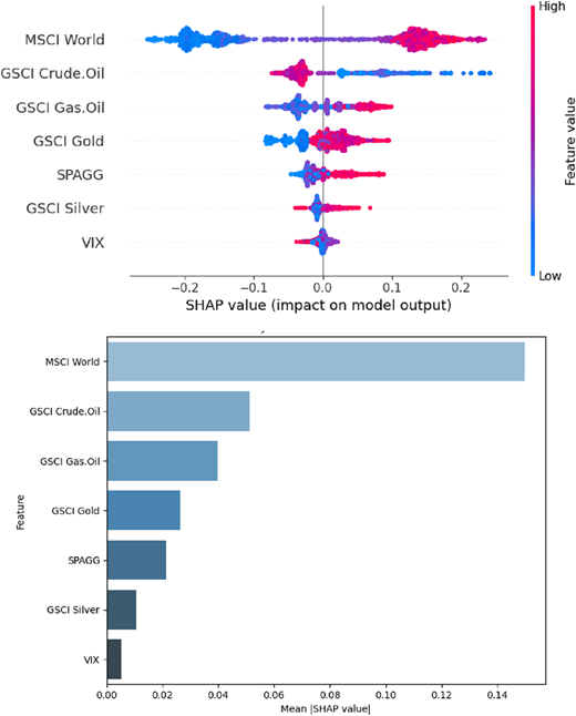
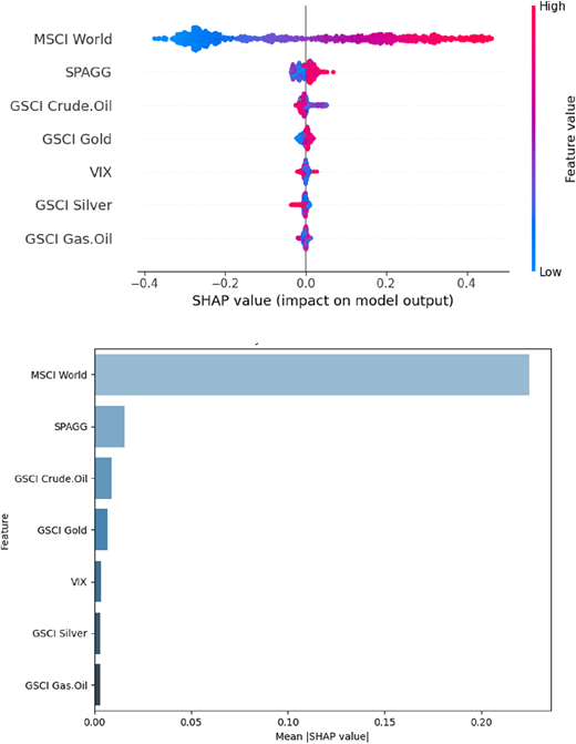
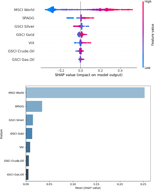
Figure 3 to 6 display the results presented in Table 4. For each index, Figure (a) shows the SHAP summary plot (beeswarm), which illustrates the distribution of Shapley values for each observation, while Figure (b) shows the average relative importance of each variable. The variables are ranked in descending order of importance on the y-axis and the Shapley values are plotted on the x-axis. In Figures (a), the color red (blue) indicates a high (low) level of the variable. For example, a positive relationship between a variable and the index is represented by red dots (high level) associated with high Shapley values and blue dots (reliable level) associated with low or negative Shapley values.

For the green bond index (SPGBI), the conventional bond index (SPAGG) is the most important variable: stronger performance in the conventional bond market leads to stronger performance in green bonds. This positive relationship between the green bond market and the conventional bond market is confirmed by the findings of Kocaarslan and Soytas (2023) and Adekoya et al. (2023). The results also indicate a negative relationship between energy prices (Gas.Oil and Crude.Oil) and green bonds: a rise in these prices reduces the predicted value. This reflects the sensitivity of the green bond market to energy shocks. A positive but relatively weak relationship is observed between silver and the green bond index.

For the Clean Energy Index (SGCEI), the MSCI World Index is the most significant variable, with a strong positive relationship: higher performance in the developed stock market leads to higher performance in the Clean Energy Index. The results indicate a negative relationship between energy prices (Crude.Oil and Gas.Oil) and the Clean Energy Index: a rise in these prices reduces the forecast, reflecting a spillover effect between the energy market and green markets. This inverse relationship is consistent with the findings of Sadorsky (2022) and Fu et al. (2022). A positive relationship is observed between gold and the clean energy index, with high gold prices associated with positive Shapley values. Conventional bonds and the VIX exhibit a positive but relatively weak relationship, with their contribution to the forecast remaining limited compared to the MSCI.World and energy prices.

For the water index (SGWI), the MSCI World Index is the most important variable, with a strong, positive relationship: higher performance in the developed market leads to higher performance in the water index. These results confirm the dominant role of the developed market in determining green indices, consistent with Ramyar and Kianfar (2019) and Mohsin and Jamaani (2023). Conventional bonds (SPAGG) exhibit a positive but relatively weak relationship with the SGWI. An ambiguous relationship is observed between Crude.Oil, gold, the VIX, silver and Gas.Oil on the one side and the water index on the other, with these variables showing a marginal contribution to the prediction.

For the environmental index (MSCI.NEV), the MSCI World Index is the most significant variable, with a positive and strong relationship: higher performance in the developed market leads to higher performance in the environmental index. This result confirms the dominant role of the developed stock market in determining green indices, consistent with Ramyar and Kianfar (2019) and Mohsin and Jamaani (2023). Conventional bonds (SPAGG) also exhibit a positive relationship, though of smaller magnitude than that of the MSCI World: high bond values are associated with negative Shapley values. A negative but weak relationship is observed between silver and the environmental index, with high silver values being associated with negative Shapley values. An ambiguous relationship is observed between gold, the VIX, Crude Oil and Gas Oil on the one side and the environmental index on the other; these variables show a marginal contribution to the prediction.

In summary, the SHAP analysis reveals heterogeneity among the four green indices. The MSCI World leads the way for SGCEI, SGWI and MSCI.ENV, with a strong positive correlation, reflecting the integration of green assets into developed equity markets. The SPGBI follows a distinct pattern, driven by the conventional bond market (SPAGG). Energy prices have a negative impact on the SPGBI and SGCEI, reflecting their sensitivity to energy shocks, whereas this effect remains ambiguous for the SGWI and MSCI.ENV. The other variables (gold, silver, VIX) have a minor role in all four cases.

After selecting the features for each variable, we proceed to model training. The hyperparameters for each machine learning and deep learning model were determined empirically based on a combination of insights from the existing literature and empirical evidence from previous studies (Dutta et al., 2020, for the recurrent models; Breiman, 2001; Chen and Guestrin, 2016; Ke et al., 2017, for the tree-based models). This approach ensures that the models are configured with meaningful and effective parameter settings, tailored to our forecasting objectives and the characteristics of green asset indices. Table 5 presents the finalized hyperparameter values for all models.

Table 6 reports the performance metric results of all machine learning and deep learning models applied in this research on four indices (SPGBI, SGCEI, SGWI, MSCI.ENV). The metrics are R², MAE, MSE and RMSE. Findings indicate that the deep learning models (RNN, LSTM, GRU) generally outperform the machine learning approaches (Random Forest, XGBoost, LightGBM) in prediction. For the SPGBI, all models show strong predictive accuracy, with R² values exceeding 0.90. The GRU model achieves the highest power (R² = 0.9493) and the lowest forecast errors, indicating its capacity to model the complex dynamics of green bond prices. Concerning the SGCEI, the findings indicate that the RNN achieves the highest predictive accuracy (R² = 0.9194), suggesting that a simple recurrent structure is particularly effective in capturing the temporal dynamics of carbon-efficient assets. Concerning the SGWI, all models demonstrate outstanding accuracy (R² > 0.96), confirming the high predictability of global green indices. The GRU slightly outperforms the other approaches (R² = 0.9839), followed closely by the LSTM, emphasizing the advantage of recurrent architectures in modeling sequential dependencies. For the MSCI.ENV index, the GRU achieves the highest R² (0.9395), while the Random Forest shows strong predictive ability (R² = 0.9559), confirming its effectiveness in modeling nonlinear relationships without strong temporal effects. This result corroborates Sadorsky (2022) and Qian and Zhang (2025) findings that Random Forest performed well in forecasting stock prices, particularly clean energy ETFs and large S&P 500 firms.

The GRU model generally provides strong forecasting performance. In fact, for SPGBI, it achieves R² = 0.9493 with the lowest MAE and RMSE (MAE = 0.0114, RMSE = 0.0138) and delivers excellent results for SGWI (R² = 0.9839) and MSCI.ENV (R² = 0.9395). The results confirm that the GRU model can represent time-dependent structures related to financial asset forecasting. This result is consistent with previous research. Zhao et al. (2021) and Hamayel and Owda (2021) found that the GRU produced higher accuracy than LSTM models for stock and cryptocurrency forecasting. Also, Drira et al. (2025) showed that the GRU outperformed conventional methods for agricultural commodity price prediction.

Overall, deep learning models, especially the GRU architecture, generally present effective forecasting performance. However, the optimal model depends on the specific green asset under consideration, suggesting that forecasting effectiveness is asset-specific rather than universal.

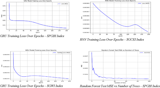
To assess the suitability of the selected models (GRU, RNN and Random Forest) for predicting green assets, we examine their learning process and predictive performance. Figure 7 shows the training progression of the three models across selected green assets.

The GRU model exhibits a decreasing MSE over epochs for the SPGBI and SGWI indices, indicating that it updates its parameters during training and effectively captures sequential structures in the data. The RNN model also shows a gradual reduction in MSE for the SGCEI index, confirming its ability to model temporal dependencies in financial time series. The Random Forest model decreases the test MSE as the number of trees increases for the SPGBI index, reflecting progressive improvement in predictive accuracy, which stabilizes after a sufficient number of trees.

Overall, these trends confirm the reliability and robustness of the selected models in forecasting green assets. Collectively, the results provide empirical evidence that the chosen models effectively learn underlying patterns in the data and produce accurate predictions, supporting their suitability for forecasting financial indices and green assets.

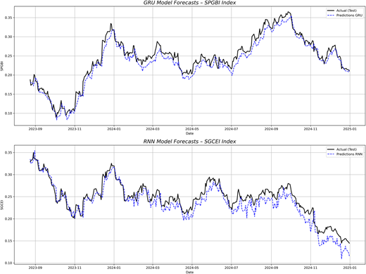
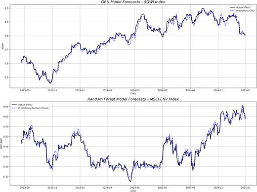
Following the assessment of model performance, we plot the forecasted values for each green asset. Figure 8 shows the comparison between actual values and forecasts for each green asset over the test period. We forecast SPGBI and SGWI using GRU, SGCEI using RNN and MSCI.ENV using Random Forest.

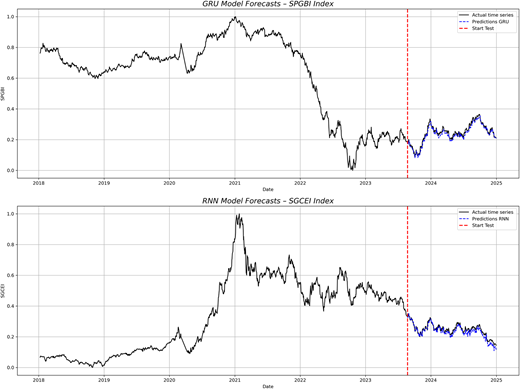
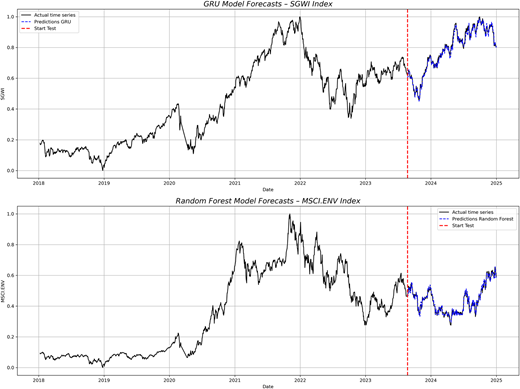
Figure 9 shows the full time series, covering both training and test periods and overlays forecasts on the test portion to demonstrate how each model tracks the overall data. The black line represents the complete actual time series (train + test), while the blue dashed line shows the predictions during the test period. The red vertical lines denote the beginning of the test phase.

As observed, the GRU model closely tracks the true values, accurately capturing the underlying patterns and dynamics of each index. This strong correspondence between predicted and observed values highlights the model's robust forecasting capability, consistent with the high R² values and low error metrics reported in Table 6. In particular, the GRU model demonstrates robustness in adapting to diverse market behaviors across all four indices. These graphical results further support the conclusion that the GRU model generally achieves high forecasting accuracy in the context of sustainable finance. Furthermore, the GRU model's simple design allows it to learn time-related patterns effectively while requiring less computational power than more complex alternatives, such as the LSTM. This makes it a practical choice for datasets of moderate size, where both accuracy and efficiency are important. Its performance across the four indices, affected by different market factors, shows the model's ability to adapt to different scenarios and capture relationships in the data. These results are consistent with Dutta et al. (2020), who found that GRU can be used for forecasting financial time series.

This study investigates the forecasting of four green asset prices, including green bonds, clean energy, water and environmental sector indices, using machine learning and deep learning models. We aim to assess the impact of stock markets and commodities on these assets; therefore, we select the MSCI World Index, the VIX and the S&P U.S. Aggregate Bond Index as stock market indicators and the S&P GSCI Gold, S&P GSCI Silver, S&P GSCI Crude Oil and S&P GSCI Gas Oil as commodity indices. The analysis relies on daily data from January 2018 to December 2024, comparing machine learning algorithms (Random Forest, XGBoost, LightGBM) with deep learning architectures (RNN, LSTM, GRU).

The use of SHAP (Shapley Additive Explanations) enables understanding the factors influencing each index. This approach enhances the interpretability of complex model predictions and provides valuable insights for identifying key indicators. The findings highlight major factors, such as the S&P U.S. Aggregate Bond Index and the MSCI World Index, as significant drivers for almost all green assets. For green bonds, traditional bond markets and gas oil prices exert the strongest impact. Clean energy prices primarily reflect the influence of developed stock markets and crude oil prices. The water and environmental indices mainly depend on developed equity markets and bond prices. These results indicate that green indices remain sensitive to traditional financial and energy markets. Furthermore, the study offers investors practical tools to manage risk and identify potential opportunities.

Empirical results showed that deep learning models, especially the GRU architecture, generally deliver high forecasting performance. By effectively capturing sequential dependencies in the data, these models provide a more accurate representation of market dynamics than static machine learning approaches. The performance of the selected models is evaluated using multiple metrics (R², MAE, MSE, RMSE), confirming the reliability and robustness of these models, with predicted prices closely matching actual values during both training and testing periods. However, the optimal model varies across green assets, suggesting that forecasting effectiveness is asset-specific rather than universal.

These results contribute to the literature by demonstrating the value of integrating deep learning models into green asset price forecasting. Deep learning approaches, especially GRU, prove particularly effective in handling the complexity and volatility of these assets. Accurate forecasts of green financial indices can support portfolio diversification, optimize capital allocation and assist in hedging strategies. As a result, investors and portfolio managers can reduce risks while enhancing returns through improved decision-making.

The findings provide valuable insights for policymakers aiming to promote sustainable finance. Understanding the key drivers of green financial indices can guide the design of regulatory frameworks and incentive mechanisms that support green investments. For instance, measures in conventional bonds and developed equity markets may influence the performance of green assets. Moreover, identifying the sensitivity of green indices to energy and commodity prices highlights the need for integrated policies that consider environmental and financial market interactions. These insights can help in developing strategies to encourage capital allocation toward sustainable sectors while managing systemic risks. This study also gives practical insights for investors and portfolio managers involved in sustainable finance. The high forecasting performance of deep learning methods, particularly GRU, suggests that financial institutions can achieve better prediction accuracy and make better investment decisions by integrating advanced data-driven methods into their analytic framework.

This research contributes to the literature. Future studies may examine hybrid machine learning approaches to improve the prediction of green asset prices. In addition, analyzing other variables, such as climate indicators, could provide insight into the factors affecting green assets.

The authors would like to thank the editors and reviewers for their helpful comments.