

This paper aims to analyze the impact of Covid-19 on the stock market volatility and uncertainty during the first and second waves.
This study has applied event study and autoregressive integrated moving average models using daily data of confirmed and death cases of Covid-19, US S&P 500, volatility index, economic policy uncertainty and S&P 500 of Bombay Stock Exchange to attain the purpose.
It is observed that, during the first wave, the confirmed cases and the fiscal measure have a significant impact, while the vaccination initiative and the abnormal hike of confirmed cases have a significant impact on the US stock returns during the second wave. It is further observed that the volatility of Indian and US stock markets spillovers during the sample period. Moreover, a perpetual correlation between the Covid-19 and the stock market variables has been noticed.
At present, the world is experiencing the third wave of Covid-19. This paper has considered the first and second waves.
It is expected that business leaders, stock market regulators and the policymakers will be highly benefitted from the research outcomes of this study.
This paper briefly highlights the drawbacks of existing policies and suggests appropriate guidelines to successfully implement the forthcoming initiatives to reduce the catastrophic impact of Covid-19 on the stock market volatility and uncertainty.
1. Introduction
The response of stock market against an event depends on its nature (Becchetti and Ciciretti, 2011). Previous studies observed the reactions of stock market against different events. Goel et al. (2017) observed negative impact of terrorist incidents. Guo et al. (2020) found a positive impact of favorable environmental policies on stock return. Lee and Chen (2020) noticed adverse impact of natural disasters and geopolitical risks on cross border exchange traded funds. Hussain and Ben Omrane (2020) found significantly positive effect of announcement of US macroeconomic news on the Canadian stock market. Curatola et al. (2016) observed positive sentimental impact of world cup games on the sectoral stock return. Hillier and Loncan (2019) detected negative impact of political uncertainty on the stock market return in Brazil. There are evidence that stock market reacts to pandemic diseases like severe acute respiratory syndrome outbreak (Chen et al., 2007), Ebola outbreak (Ichev and Marinč, 2018) and Covid-19 (Chowdhury et al., 2021). Originating from the Wuhan city in China (Alanagreh et al., 2020), the devastating coronavirus diseases widely known as Covid-19, has traveled across the world taking 3,311,780 lives and infecting 159,319,384 people as of May 13, 2021 [1]. The World Health Organization (WHO) officially announced Covid-19 as a pandemic on January 30, 2020 (WHO, 2020). Along with health hazards, this virus severely destroyed the world economy causing job loss, winding up of business and enlarging the size of low-income people (Mottaleb et al., 2020; Maital and Barzani, 2020; Ibn-Mohammed et al., 2020; Chowdhury, 2020). Realizing the massive impact of this virus on global economy, Gates (2020) treats the virus as “the once-in-a century pathogen”. The instant impact of Covid-19 was clearly observed in the sharp fall of major three US indices such as S&P 500, NASDAQ and the Dow Jones Industrial Average (Chowdhury, 2017; Albulescu, 2021). The fall continued until the US government passed Coronavirus Aid, Relief and Economic Securities (CARES) Act and subsequently the three indices jumped by 7.3%, 7.33% and 7.73%, respectively (Corbet et al., 2020). The impact of Covid-19 has been measured on different areas such as oil price and the UK economic policy uncertainty (EPU) (Jeris and Nath, 2020), geopolitical ramification in Taiwan (Zhang and Savage, 2020), economics (McKibbin and Fernando, 2020), agriculture (Siche, 2020), school closure and academic achievement (Kuhfeld et al., 2020), environment (Wang and Su, 2020) and psychology (Dubey et al., 2020). While Yousfi et al. (2021) measured the impact on US stock market comparing the first and second wave using auto regressive moving average dynamic conditional correlation generalized autoregressive conditional heteroskedasticity, this study applies event study and auto regressive integrated moving average (ARIMA) in comparison with standard and poor (S&P) 500 index of Bombay Stock Exchange.
Discovering the nature of impact on US stock market in two different periods is the main motivation behind this study. Financial volatility derives from various sources such as institutional affairs, market uncertainty, economic conditions and macroeconomic announcements (Chowdhury et al., 2022; Hartwell, 2018). Onan et al. (2014) found asymmetric impact of good and bad announcement on the financial volatility. The EPU most often play an important role in influencing the financial volatility (Chen and Chiang, 2020; Li et al., 2020).
This study aims to measure the impact of four Covid-19 events such as confirmed cases, fiscal measures, vaccination and abnormal rise of confirm cases on the US stock market as well as to establish volatility spillover model by investigating the conditional correlations between the US and Indian stock indices during first and second waves of Covid-19. The contributions of this paper are in two folds. First, the impact of Covid-19 confirmed and death cases on US stock indices and economic uncertainty during first and second waves separately and second, the nature of spillover risk between US and Indian stock markets during first and second waves.
This study observes a significantly negative impact of Covid-19 on the US stock market being an idiosyncratic black swan event. While ARIMA negatively predicts the S&P 500, the Dynamic Conditional Correlation (DCC) senses the contagion effects with the increasing trend of death and confirmed cases in the US.
2. Literature review
Most of the studies focus on the impact of financial events on the stock market while very few studies are based on the negative impact of public health like influenza and pandemic. McTier et al. (2013) noticed the opposite direction of increase in number of flu and stock market return in the US stock market. Goh and Law (2002) observed terrific impact of Asian financial crisis in 1997 and avian influenza outbreak in 1998 on the tourism sector in Hong Kong. Chen et al. (2007) found the stock prices of hotel industry in Taiwan went down to the lowest level due to the SARS. Similarly, Covid-19 influenced the Asian financial market (Narayan and Phan, 2020), global economy (Iyke, 2020), aviation industry and employment (Sobieralski, 2020), crude oil prices and stock returns (Liu et al., 2020). Ewing et al. (2006) observed quick effect of hurricane on the US economy. They further noticed that the affect lasted for some time. Lamb (1998) and Angbazo and Narayanan (1996) found severe impact of hurricane on the stock prices of insurance companies. Even heavy wind speed and landfall (Ewing et al., 2006), inappropriate mergers (Chowdhury, 2012) reduces the share prices significantly. There exists a relationship between natural calamity and stock market performance. The irregular supply of energy like power, water and gas hampers production process or service delivery of a company thus it reduces the share price of that company (Hallegatte and Dumas, 2009). Jaussaud et al. (2015) detected a significantly negative impact of tsunami on the stock prices and different industries in Japan. Although Yousfi et al. (2021) studied the impact of first and second waves of Covid-19 on the US stock market, they did not apply the event study method. This study will fill the gap by applying event study method in assessing the impact of two events during first and second wave respectively.
Apart from different events, a stock market is influenced by socioeconomic and financial factors. Baker et al. (2020a, b) investigated the impact of Covid-19 on the Eurasian and US stock market. Akhtaruzzaman et al. (2021a) observed a significant shift in the conditional correlations between the stock returns of China and G7 economies among the financial and nonfinancial firms. Corbet et al. (2020) found China as the epicenter of both physical and financial contagion. Due to negative impact of Covid-19, investors have lost their capital in the short-run and the risk level in financial market has reached at the peak (Zhang et al., 2020). Using high frequency data, Akhtaruzzaman et al. (2021a, b, c, d) observed that gold acts as a secured investment sector during Covid-19 pandemic specially the second wave.
The pandemic has high impact on the economic uncertainty at every level of economy. Ashraf (2020) noticed a negative impact of increasing confirmed cases on the stock market return. He also observed that death cases have less impact than confirmed cases on the stock markets. Sharif et al. (2020) observed higher impact of Covid-19 on the geopolitical risks than that of economic uncertainty in the US by applying wavelet approach. Media coverage index and ESG leader indices are found highly connected to the US stock market (Akhtaruzzaman et al., 2021a, b, c, d). The impact of Covid-19 on the policy responses is significantly positive in 67 countries. Although pharmaceutical industry made profit, rest of the sectors experienced tremendous volatility in their stock prices (Zaremba et al., 2020). The regular bulletin on confirmed cases of Covid-19 makes US financial market significantly volatile (Albulescu, 2021). He further mentioned that long-lasting nature of Covid-19 plays a vital role in enhancing the volatility of stock market and thus turns risk-management pretty difficult. The negative impact of Covid-19 pandemic has heavily been observed on the oil price exposure of both financial and non-financial industries (Akhtaruzzaman et al., 2021a, b, c, d). Goodell (2020) studied a comparative relationship between Covid-19 vs. economic activities and natural disaster vs. economic activities. He found the effect of Covid-19 on economic activities is more severe than that of natural disasters namely nuclear war, climate change and environment pollution. During the first wave, the economic activities went down due to shortage of labor supply, low production of goods and services fearing the spread of virus (The Economist, 2020). The attack of Covid-19 on US financial market is heavier than the financial crisis of 2008 although this market was not as strong as organized today. Apart from increasing number of confirmed cases, the restrictions imposed by the US government on movement made the market more volatile (Harvey, 2020). Abdelkafi et al. (2022) analyzed the relationship between government actions and Covid 19 pandemic in 10 American and Latin countries. They observed negative impact of coronavirus on stock prices and behavior of investors while governments’ financial support played a positive role in reducing the negative impact of the same. Priscilla et al. (2022) noticed adverse impact of confirmed cases and deaths on the stock market liquidity; on the contrary, vaccinations and recovery news had positive impact in four ASEAN capital markets. Yarovaya et al. (2022) observed a contagion effect and intraregional and interregional return and volatility spillovers based on four levels of information transmission such as catalyst of contagion, media attention, spillover effect at financial markets and macroeconomic fundamentals.
The above review covers the latest developments on the impact of events and socioeconomic factors on different sectors. The following section investigates the effect of four pandemic events through event study method and constitutes appropriate econometric models to analyze the impact of Covid-19 on the US stock market and uncertainty during the first and second waves separately.
3. Data and models
3.1 Data
To achieve the objectives, the daily US S&P 500 index which represents top 500 large companies in the US stock market and Indian BSE S&P 500 index which also represents top 500 large companies in Indian stock market have been considered from January 1, 2015 to April 22, 2021. The US volatility index (VIX) that indicates the stock market’s volatility over the next 30 days, [2] EPU that measures the uncertainty of a country based on the newspaper references focusing on the differences among the economic forecasters regarding policy variables and uncertainty (Baker et al., 2020a, b) and Covid-19 variables, namely total confirmed cases and total deaths have been considered from January 1, 2020 to April 22, 2021 (see Figure 1).
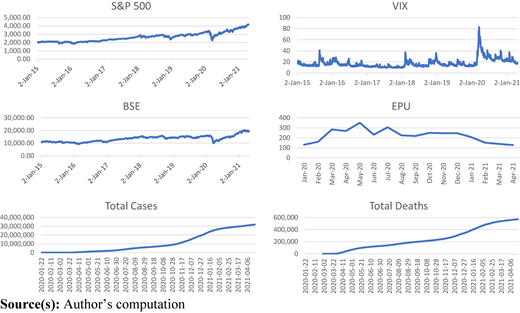
Time series data of US S&P 500, US VIX, BSE S&P 500, EPU, total confirmed cases and total death cases
Time series data of US S&P 500, US VIX, BSE S&P 500, EPU, total confirmed cases and total death cases
The period for the event study ranges between 1 January, 2015 to April 22, 2021 and the events include first confirmed case on 21 January, 2020, the day when US government announced financial bailout on 6 March, 2020 (Chowdhury et al., 2021), first vaccination in the US on 14 December, 2020 (Ben et al., 2020) and the first abnormal case right after first wave was recorded on 14 October 2020 (James et al., 2021). The stock indices have been collected from the investing.com [3] and the Covid cases have been collected from the website of WHO [4].
3.2 Models
3.2.1 Event study method
Event study is a research approach in finance widely used to examine the effects of an incident such as merger, dividend announcement, financial or health crisis and change of key personnel by verifying the responses of the stock price around the occurring of the event (Chen et al., 2007). This method measures the abnormal changes of stock prices or abnormal returns (ARs) after an occurring event. The process is based on the finance theory, of efficient capital market, that the capital market reflects all the information about an event on the stock prices (Fama et al., 1969; Schimmer, 2012). The Covid-19 is such an event that has created panic among the people across the world and influences the capital market instantaneously. Being a highly sensitive market, employment of an event study will give a genuine scenario of the Covid-19’s impact on the US stock market. This study analyzes the impact of Covid-19 focusing on four major incidents as mentioned earlier. To observe the behavior of AR during the first and second wave, T-test has been used.
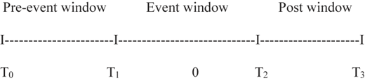
Figure 2 shows different windows of event study. Pre-event window covers the normal period prior to the event day. Based on the data of this period, both intercept and slope of the asset valuation model have been computed to estimate ARs after the event day. Based on the availability of Covid-19 data, the pre-event period starts from January 1, 2020. Event window is the day when an event takes place and post-event window is the period starts right after the event day.
ARs may be computed following three approaches such as the market index adjusted rate of return, the market model and the average adjusted rate of return. On an event day, when market becomes either bull or beer, the significant deviation is observed if the average adjusted rate of return model is applied (Klein and Rosenfeld, 1987). While, the market index adjusted return model is significantly based on assumption (Huang and Li, 2018), the market model is widely used model that can estimate far better way than others (Brenner, 1979).
This study employs the market model as follows:
The normal return is computed as the following:
where, is the expected return of ith stock on day t, measures systematic risk and is the market return on day t. is the statistic disturbance. The intercept and beta have been computed based on the data of pre-event period. Putting the value of and on Eq. (1), the AR is calculated as below:
, and refer to expected return, real return and AR of index I on t day within post-event window. When ARs are added over the time, the cumulative abnormal returns (CAR) are obtained as below:
Here, t refers to time frame.
3.2.2 Auto regressive integrated moving average (ARIMA)
The daily stock returns have been computed applying the following formula:
here pt represents the daily closing prices. This study measures the stock market volatility spillover using ARIMA and auto regressive moving average dynamic conditional correlation generalized autoregressive conditional heteroskedasticity (ARMA–DCC–GARCH) models. These models can appropriately examine the time-varying correlations between economic variables and the financial products (Ciner et al., 2013). The ARMA (1, 1) model is represented by the following equation:
where, rt is stock return and is residual. The residuals can be modeled by:
where, Ht derives as the conditional covariance matrix from Rt and zt is the vector of nx1. After estimating GARCH parameter, the DCC is estimated in the following step using the following equation:
where, Ht represents the conditional covariance modeled in n x n matrix, Rt represents conditional correlation matrix while Dt represents a diagonal matrix of time-varying standard deviations. The Rt and Dt are determined as follows:
here, h represents the universe of GARCH models, applied to generate the value of h on the diagonal matrix. Therefore, the parameters of Ht of GARCH model are derived in the following way:
The symmetric positive matrix of Qt is written by:
where Q represents the unconditional correlational matrix of the standardized residuals. In order to establish DCCs, both a and b are used in smoothing process. If a+b is less than unity, that is, [(a+b) < 1] and positive, it indicates, the DCC model returns to equilibrium. Thus, the correlation is determined as follows:
Goodness of fit has been tested by using Akaike information criterion (AIC) and Bayesian information criterion (BIC). The models are used to balance the intricacy of the model and the model fit. The equations are given below:
where L represents the value of the likelihood function, N indicates the number of observations and k denotes number of estimated parameters.
4. Empirical findings and discussion
Table 1 exhibits the descriptive summary of the data used in this study. The skewness is positive for all the variables except US S&P 500 of the second wave. The kurtosis values indicate the variables are normally distributed except for US VIX and US S&P 500 as the values are less than 3.
Descriptive summary of VIX, S&P 500, BSE, EPU and Covid-19 cases/deaths
| VIX | S&P 500 | BSE | EPU | CC | DC | |
|---|---|---|---|---|---|---|
| First wave | ||||||
| Mean | 17.716 | 2644.730 | 13480.490 | 22.106 | 3.035 | 1.946 |
| Med | 15.175 | 2638.700 | 13928.900 | 22.024 | 0.000 | 0.000 |
| Std. Dev. | 8.159 | 526.612 | 2353.573 | 0.291 | 5.029 | 3.745 |
| Kur | 13.374 | −0.146 | 0.041 | 1.102 | −0.003 | 0.700 |
| Skew | 2.902 | 0.672 | 0.475 | 0.828 | 1.324 | 1.573 |
| Min | 9.140 | 1829.080 | 9187.970 | 20.983 | 0.000 | 0.000 |
| Max | 82.690 | 4185.470 | 20305.800 | 22.925 | 13.804 | 10.937 |
| Obs | 1592 | 1587 | 1558 | 363 | 363 | 363 |
| Second wave | ||||||
| Mean | 0.006 | 2767.186 | 19.519 | 22.070 | 2.353 | 1.368 |
| Med | −0.006 | 2719.248 | 19.443 | 22.001 | 0.000 | 0.000 |
| Std. Dev. | 0.096 | 587.69 | 0.377 | 0.277 | 4.352 | 3.137 |
| Kur | 5.149 | −0.245 | 3.314 | 2.086 | 1.425 | 3.028 |
| Skew | 1.694 | −0.547 | 1.337 | 0.975 | 1.722 | 2.137 |
| Min | −0.234 | −1925.32 | 18.272 | 20.983 | 0.000 | 0.000 |
| Max | 0.465 | 4985.14 | 21.508 | 22.925 | 13.804 | 10.937 |
| Obs | 306 | 306 | 306 | 306 | 306 | 306 |
Source(s): Author’s computation
Table 2 shows, though during the first wave, US VIX has negative correlation with other variables, in the second wave it has positive correlation with all except the US S&P 500. During the first wave, the VIX index was negatively influenced as the death by Covid-19 was recognized only after diagnosis of Covid 19. Therefore, the increasing number of death cases resulted in the decreasing trend of VIX index (Grima et al., 2021). On the other hand, US S&P 500 has positive correlation with all the variables during first wave but it has negative correlation with all except death case. However, other variables are positively correlated. Chowdhury and Abedin (2020) and Mei et al. (2019) also noticed the similar relations.
Correlation coefficient between the variables during first and second waves
| VIX | S&P 500 | EPU | BSE | CC | DC | |
|---|---|---|---|---|---|---|
| First wave | ||||||
| VIX | 1 | |||||
| S&P 500 | −0.62 | 1 | ||||
| EPU | −0.07 | 0.05 | 1 | |||
| BSE | −0.04 | 0.03 | 0.90 | 1 | ||
| CC | −0.02 | 0.06 | 0.80 | 0.70 | 1 | |
| DC | −0.05 | 0.09 | 0.78 | 0.68 | 0.98 | 1 |
| Second wave | ||||||
| VIX | 1 | |||||
| S&P 500 | −0.69 | 1 | ||||
| EPU | 0.12 | −0.08 | 1 | |||
| BSE | 0.17 | −0.09 | 0.88 | 1 | ||
| CC | 0.04 | −0.01 | 0.76 | 0.68 | 1 | |
| DC | 0.00 | 0.01 | 0.75 | 0.66 | 0.97 | 1 |
Source(s): Author’s computation
Table 3 indicates, during the first wave, the market responded significantly negative on the very next day at the news of first confirmed case on 21 January, 2020 (although not shown in the table) and continued throughout the month. Ashraf (2020) observed the US stock market return was declining along with the increased number of cases. In that week, the Dow Jones Industrial Average dropped by 622 points, NASDAQ composite index dropped by 284 points and the S&P 500 dropped by 81 points. The impact was so terrific that Apple was forced to withdraw their revenue guideline as there was shortage of products due to supply crisis in China. The opposite reaction was observed in the case of Amazon, as people stopped visiting physical market, the revenue of Amazon jumped by 37% within the first three months which fetched them nearly $96.15 billion profit and created 250,000 new jobs (Helmore, 2020). Yong and Laing (2021) found both short-run and long-run negative impact of Covid-19 on exports, imports, sales and productions along with stock market returns. When the US government announced the financial bailout, the response of market was not positive instantly, rather it took a few days to be positive although there were ups and down as the news failed to restore the fear of investors (Elenev et al., 2020).
Cumulative abnormal returns before, during and after the detection of Covid-19 case and announcement of fiscal measure during first and second waves
| Event window | First wave | Second wave | ||
|---|---|---|---|---|
| First confirmed case | Fiscal measure | First vaccine | Abnormal confirmed case | |
| (−30, 0) | 1.241616*** (4.869601) | −0.61755*** (−102.871) | 0.192782*** (27.18336) | −0.02298*** (−3.12826) |
| (−25, 0) | −1.54057*** (−6.0421) | 0.145511*** (24.23929) | −0.29989*** (−42.2864) | 0.183398*** (24.96058) |
| (−20, 0) | 0.757862*** (2.972323) | −0.23353*** (−38.901) | 0.180864*** (25.50287) | −0.03381*** (−4.60211) |
| (−15, 0) | 0.081909 (0.321246) | −0.35166*** (−58.5801) | 0.681387*** (96.07952) | 0.756385*** (102.9445) |
| (−10, 0) | 0.149358 (0.585779) | 0.337485*** (56.21841) | 1.421493*** (200.4386) | 0.287239*** (39.09343) |
| (−5, 0) | −1.18755*** (−4.65757) | −0.50498*** (−84.1198) | 0.539838*** (76.12028) | 1.060435*** (144.3259) |
| (0, 0) | 1.503026*** (5.894849) | 0.822993*** (137.0947) | −1.26174*** (−177.912) | 0.11347*** (15.4434) |
| (0, +5) | −0.93067*** (−3.65007) | 0.278572*** (46.40471) | 0.636912*** (89.80827) | 1.552299*** (211.2689) |
| (0, +10) | 0.16981 (0.665991) | 0.194695*** (32.43245) | 0.236952*** (33.41152) | 0.754823*** (102.732) |
| (0, +15) | −0.95757*** (−3.75558) | 0.612704*** (102.0647) | −0.23627*** (−33.3159) | −2.06196*** (−280.634) |
| (0, +20) | −0.74891*** (−2.93723) | −0.92107*** (−153.432) | 0.664407*** (93.68514) | 0.97552*** (132.7689) |
| (0, +25) | 0.201963 (0.792095) | 0.119963*** (19.98349) | 0.224794*** (31.69724) | −2.07841*** (−282.874) |
| (0, +30) | −0.40677 (−1.59533) | −0.58541*** (−97.5184) | 0.374318*** (52.78092) | −0.08063*** (−10.9738) |
Note(s): Figures within parenthesis represent t-values. The ordinate indicates the even window. ***, ** and * are the significant at 1%, 5% and 10%, respectively
Source(s): Author’s computation
When the first Covid-19 vaccine was pushed for the first time on 14 December, 2020, the reaction of the US market was significantly positive. The subsequent success news of corona vaccine manufactured by AstraZeneca – Oxford, Pfizer – BioNTech and Moderna positively influenced the market (COVID-19: Impact of vaccines on the stock market, 2021). From 23 July to 13 October, both the number of infection and death cases were reducing but when the rate started to spike from 14 October, 2020 the market did not respond to it negatively, rather the index was climbing up. The index of S&P 500 increased by 65% since March 2020 while that of NASDAQ increased by 44%. The second wave could not tarnish the market like the first wave as people started to work from home, children started taking lessons through online mode, service organizations introduced home services following the guidelines prescribed by the WHO. The stable fiscal and monetary policy along with approval of stimulus packages worth $500 to $1 trillion convinced the investors to hold their stocks (Domm, 2020a). The updates on the successful trials of corona vaccines also played a vital role to safeguard the market (Domm, 2020b).
In this study, the ARIMA model has been applied following four steps such as identification, estimation, diagnosis checking and forecasting. The appropriate model has been identified by applying correlogram, Autocorrelation function (ACF) and partial autocorrelation fiction (PACF). correlogram has been used to select appropriate lags for AR and moving average (MA) by plotting ACFs and PACFs against lag length. Figure 3 indicates that the line plot of both S&P 500 and BSE series are stationary.
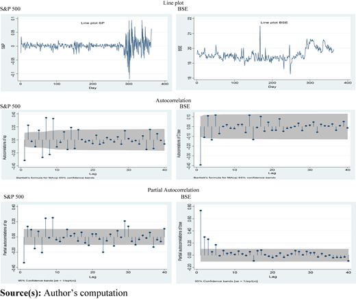
However, the Augmented Dickey Fuller (ADF) and Phillip–Perron (PP) unit root results (Table 4) also give the same results. Though the S&P 500 and VIX are stationary at first difference under ADF during the first wave, the rest of the variables are stationary at level during both first and second waves.
Unit root test results
| S&P 500 | VIX | EPU | BSE | |
|---|---|---|---|---|
| First wave | ||||
| ADF | −26.946*** (I) | −21.315*** (I) | −7.033*** (o) | −8.313*** (o) |
| PP | −23.123*** (o) | −23.195*** (o) | −4.856*** (o) | −7.117*** (o) |
| Second wave | ||||
| ADF | −25.886*** (o) | −19.735*** (o) | −5.635*** (o) | −7.482*** (o) |
| PP | −24.656*** (o) | −19.594*** (o) | −5.063*** (o) | −7.409*** (o) |
Source(s): Author’s computation
The first wave data of S&P 500 and BSE have been converted to first deference to make them suitable for the model. The autocorrelation results indicate that most of the spikes are within the shed while only one lag of BSE and two lags of S&P 500 are outside the shed, thus the series are AR progress. From the associated correlogram of ACF and PACF, this study selects ARIMA (1, 1, 1) and ARIMA (1, 1, 2) models. Table 5 exhibits the estimates of four models for S&P 500 and BSE under ARIMA (1, 1, 1) and ARIMA (1, 1, 2).
Estimates for the ARIMA
| (1) | (2) | (3) | (4) | |
|---|---|---|---|---|
| S&P 500 | S&P 500 | BSE | BSE | |
| main | 0.0000165 | 0.0000158 | 0.000582 | 0.000514 |
| (0.0000414) | (0.0000382) | (0.00418) | (0.00473) | |
| ARMA | ||||
| L.ar | −0.358*** | −0.505*** | 0.176*** | −0.669*** |
| (0.0235) | (0.0618) | (0.0457) | (0.143) | |
| L.ma | −0.949*** | −0.786*** | −0.777*** | 0.0814 |
| (0.00905) | (0.0651) | (0.0479) | (0.148) | |
| L2.ma | −0.164* | −0.567*** | ||
| (0.0655) | (0.0826) | |||
| Sigma | 0.0189*** | 0.0188*** | 0.241*** | 0.240*** |
| (0.000307) | (0.000312) | (0.00359) | (0.00441) | |
| N | 362 | 362 | 362 | 362 |
| AIC | −1834.687 | −1835.002 | 6.565275 | 3.694477 |
| BIC | −1819.12 | −1815.544 | 22.13185 | 23.1527 |
| Df | 4 | 5 | 4 | 5 |
| Log-likelihood | 921.3433 | 922.501 | 0.71736 | 3.152762 |
Note(s): Standard errors in parentheses * p < 0.05, **p < 0.01 and ***p < 0.001
Source(s): Author’s computation
The appropriate model is comprised with most significant coefficients, the lowest sigma square (coefficient of volatility), highest log-likelihood statistics and lowest AIC and BIC. Considering the characteristics, the ideal model for S&P 500 is the model 2 and that of BSE is the model 4. Model 2 shows both AR and MA are negative and statistically significant at 1% level, thus ensures that they can negatively predict the S&P 500. Model 4 similarly indicates that the ARIMA coefficients are significantly negative except the volatility. The diagnostic results in Figure 4 indicate the lags of S&P 500 and BSE are flat and all information are captured.
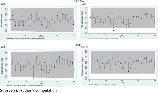
Although only one lag is significant, the parsimony is the watchword and can be ignored (Wooldridge, 2009). Thus, the ARIMA (1,1,2) is the best fitted model. Table 6 shows the contagion effect of Covid-19 on the US stock market and uncertainty during the first and second waves. The DCC process ensures the persistence of correlation between first and second waves. The coefficients of a and b are positive and significant and their sum is also less than 1 thus, ensures the return to equilibrium of DCCs. Therefore, it is observed that the volatility of returns during the first and second wave has significant impact on the dynamic relationship between the S&P 500, the VIX, the EPU and the Covid-19 variables.
DCC parameters between the US stock market, US uncertainty and the COVID-19 pandemic
| First wave | Second wave | ||||||
|---|---|---|---|---|---|---|---|
| S&P 500 | VIX | EPU | S&P 500 | VIX | EPU | ||
| a | 0.00166** | 0.0461*** | 0.0427*** | a | 0.0119* | 0.0485*** | 0.0369*** |
| (0.000987) | (0.00183) | (0.00883) | (0.00493) | (0.00235) | (0.00926) | ||
| b | 0.00251** | 0.0176** | 0.00465*** | b | 0.00209** | 0.0158* | 0.0167*** |
| (0.00132) | (0.00616) | (0.0119) | (0.00134) | (0.00684) | (0.0128) | ||
Note(s): Standard errors in parentheses * p < 0.05, **p < 0.01 and ***p < 0.001
Source(s): Author’s computation
The positive and significant coefficients of b indicate that there exists a long-term relationship among the variables which resembles the findings of Yousfi et al. (2021) and Zhang et al. (2020).
Although, at this moment resolving health crisis is the top priority, there is no way to undermine the urgency to resolve the financial and social disaster. The world economy has been worsened due to continuation of lockdown, social distancing, isolation and quarantine measures across the globe for quite a long period. The disruption in the supply chain put many businesses to disappear and added many numbers to the gang of unemployed people. To rescue the falling companies and people going under the poverty line, many countries initially announced stimulus packages. Unfortunately, the scenario did not change as it was expected. Governments should have clear provision to support the workers and their families along with saving the companies. Governments should customize their stimulus packages to help business organizations as well as to save workers by reducing layoffs, protecting incomes of employees, subsiding foods, utilities so on and so forth. A comprehensive plan including business entities and the workers from diverse backgrounds irrespective of income level, educational competencies and experience will give better results. Many governments have taken providing stimulus packages as a part of their normative framework, whereas it should be given supreme care to ensure proper application of Decent Work Agenda and the 2030 Agenda to ensure sustainable development. To safeguard the interest of mass people, policy-making process of government should be in the form of social dialog so as to formulate appropriate labor market policies, strengthen social inclusion and promote a sense of common purpose. Finally, to defeat the pandemic as well as to rescue economically weak nations, it is essential to have a global consensus and a common objective of the leading financial organizations such as the World Bank, International Monetary Fund, Asian Development Bank and New Development Bank.
5. Conclusion
This study applied event study method to unearth the impact of Covid-19 on the US stock market, ARIMA model to know the effect of Covid-19 on the US stock market and uncertainty and DCC model to measure the volatility spillover between India (BSE S&P 500) and US (S&P 500) stock market. Being a distinctive black swan event, the Covid-19 has always been unknown in term of intensity, breadth and depth and thus significantly affected the US stock market. As stock market is one of the barometers of an economy, it reflects the overall economic scenario of a country. The significant impact of all the four events indicates the sensitivity of the US stock market toward Covid-19. It is observed that ARIMA coefficients negatively predict the S&P 500. The DCC detects the existence of contagion effects when the confirmed and death cases were skyrocketing in the US. It is further noticed that the volatility spillovers between the Indian and US stock markets during the sample period. The US stock market encountered severe fall in the first three weeks of March 2020 and started to improve from the first week of April 2020 onward. Although USA witnessed the first 100,000 deaths due to Covid-19 in June, 2020, Donald Trump tested Covid positive in October, US presidential election held in November, the Capitol was revolted in January, 2021 and death toll reached to a whopping 500,000 level, the market steadily kept on climbing till April 2021. Rapid measures taken by the Federal Reserve and trillion dollars stimulus injected by the Congress in the economy played vital role in this regard. Although only four events have been considered in this study, in future other Covid-19–related factors such as announcement of restrictions, international movement, restrictions on social gatherings may be considered to get a broader picture covering the third and other waves to come.
Author is grateful to anonymous reviewers and the editor for their valuable suggestions to improve the quality of the paper.
Notes
WHO Coronavirus (COVID-19) dashboard | WHO Coronavirus (COVID-19) Dashboard with vaccination data.
Funding: This paper has received no funding.
Conflict of interest: There is no conflict of interest.
