

The study aims to investigate the impact of additive manufacturing (AM) on the performance of a spare parts supply chain with a particular focus on underlying spare part demand patterns.
This work evaluates various AM-enabled supply chain configurations through Monte Carlo simulation. Historical demand simulation and intermittent demand forecasting are used in conjunction with a mixed integer linear program to determine optimal network nodal inventory policies. By varying demand characteristics and AM capacity this work assesses how to best employ AM capability within the network.
This research assesses the preferred AM-enabled supply chain configuration for varying levels of intermittent demand patterns and AM production capacity. The research shows that variation in demand patterns alone directly affects the preferred network configuration. The relationship between the demand volume and relative AM production capacity affects the regions of superior network configuration performance.
This research makes several simplifying assumptions regarding AM technical capabilities. AM production time is assumed to be deterministic and does not consider build failure probability, build chamber capacity, part size, part complexity and post-processing requirements.
This research is the first study to link realistic spare part demand characterization to AM supply chain design using quantitative modeling.
1. Introduction
Additive manufacturing (AM) research is a rapidly evolving field that pioneers, develops and matures new materials, processes and technology. While much of hype focuses on the future possibilities, AM research will continue to yield outputs that provide innovative and even disruptive approaches to planning and managing large logistics networks for both industrial and governmental organizations. Indeed, researchers, companies and the government are already working hard to develop AM technologies for these applications – these include Volkswagen, Audi and the US Department of Defense, to name a few (Essop, 2020; Office of the Vice President for Research, 2017; Department of Defense, 2016; Department of the Army, 2016; Anonymous, 2018; Prater et al., 2016, 2017; Department of the Navy, 2017; Randolph, 2019; Prater et al., 2019; Made In Space, 2019; Goldstein, 2019; Kosowatz, 2019; Piggee, 2019; Volkswagen, 2018; Vialva, 2019; Freedberg, 2019).
Advances in AM technologies provide opportunities to employ this asset not only to support everyday logistical operations but to address contingency operations and disaster management. AM technologies serve as a rapidly responsive resource to address surges in demand and address logistical shortcomings as applied in response to the COVID-19 pandemic (Stratasys, 2020) and other disaster relief efforts.
These current and future AM technologies provide an opportunity for positive disruptive change. Even with matured AM technology, large corporations and governmental agencies with global supply chains are still faced with several key questions to fully realize the benefits:
When should adding AM capability into a logistics network be considered?
If using AM, where should AM capability be located in the network?
After establishing it, how should the AM capability best be resourced, managed and employed?
This research seeks to address the first two questions presented above, within the framework of different spare part demand patterns.
Spare parts supply chains stand apart from supply chains servicing other types of materials for a variety of reasons, specifically the uncertainty of the demand patterns, criticality of parts and high customer service level requirements (Saalmann et al., 2016). Spare parts, also referred to as service or repair parts, are those that are used to support maintenance and repair operations. Demand for spare parts occurs when a component fails, requires replacement, or is scheduled for service and as such it is different from a “typical” stock keeping unit (SKU) in other supply chains (Martin et al., 2010). The resulting demand patterns for spare parts are often highly intermittent and unpredictable (Sirichakwal and Conner, 2016; Fortuin and Martin, 1999). Further amplifying the challenges in managing a spare parts supply chain is that spare parts are often considered highly critical and carry high customer service level requirements. This criticality is determined by the consequences caused by the failure of a part when a replacement is not immediately available (Huiskonen, 2001). Monetarily, these consequences can be very high such as in the aviation industry where the cost per hour of downtime can be several thousands of dollars per hour (Abbink, 2015).
Spare part service requirements and highly intermittent demand patterns present a variety of difficulties in forecasting and inventory stock control (Syntetos and Keyes, 2009). Consequently, organizations often maintain disproportionately high inventory levels and face high inventory carrying costs, much like the US Army who “accumulated billions of dollars in excess spare parts inventory against current requirements for some items and substantial inventory deficiencies in other items” (United States Government Accountability Office, 2016). Managing the tradeoffs between high inventory carrying costs and customer service levels is not a new concept in supply chain management; however, advancements in AM technologies provide new options in this field.
This paper investigates the impact of AM on the configuration and performance of spare parts supply chains. As an extension of related work in this field, this research focuses modeling efforts on spare part demand characteristics of average inter-demand interval (ADI) and squared coefficient of variation (CV2). Within the framework of the demand classification scheme proposed by Syntetos et al. (2005), this paper explores three distinct research areas. First, we briefly explore the performance tradeoffs associated with a wide range of AM-enabled network configurations. Next, we assess for which demand classification does the addition of AM technologies into a network provide the most value. Finally, we narrow our focus on two widely researched AM-enabled network configurations, centralized and distributed and compare their performance across a wide range of spare part demand patterns.
The rest of this paper is organized as follows: Section 2 reviews applicable literature and identifies gaps; Section 3 provides a high level overview of the approach and presents our methods; Section 4 details the supply chain network and assumptions; Section 5 explores the tradeoffs of various AM configurations; Section 6 compares the performance of the centralized and distributed configurations; Section 7 explores the relationship between total demand volume and relative AM production capacity, and Section 8 provides closing remarks and extensions for future work.
2. Literature review
The literature contains a number of studies that examine efficient configurations of AM-enabled supply chain networks and their associated tradeoffs. Table 1 summarizes these papers and compares them with this paper. While our approach is unique, this paper's emphasis on intermittent demand is common in spare parts supply chains (Table 1).
Previous research comparing the different configurations of a supply chain when adopting AM as related to this research
| Type | Feature | This paper | Song and Zhang (2020) | Knofius et al. (2019) | Basto et al. (2019) | Ghadge et al. (2018) | Li et al. (2019) | Khajavi et al. (2018) | Li et al. (2017) | Liu et al. (2014) | Khajavi et al. (2014) | Holmstrom et al. (2010) |
|---|---|---|---|---|---|---|---|---|---|---|---|---|
| Network | Centralized | × | – | – | – | – | × | × | – | × | × | × |
| Distributed | × | – | – | – | × | × | × | – | × | × | × | |
| Hub | – | – | – | – | – | – | – | – | – | × | – | |
| Mixed | – | – | – | – | – | × | – | – | – | – | – | |
| Method | Conceptual | – | – | – | – | – | – | – | – | – | – | × |
| Analytical | – | × | – | – | – | – | – | – | × | – | – | |
| Simulation | – | – | – | – | – | × | – | – | – | – | – | |
| Systems dynamics | – | – | – | – | × | – | – | – | – | – | – | |
| Scenario model (Monte Carlo) | × | – | – | – | – | – | × | – | – | × | – | |
| Optimization (MILP) | × | – | – | × | – | – | – | – | – | – | – | |
| SPSC | General | × | × | – | – | – | – | – | – | × | – | × |
| Aircraft | – | – | – | – | × | – | × | – | – | × | – | |
| Maintenance | – | – | – | × | – | – | – | – | – | – | – | |
| Metrics | Inventory holdings | × | – | – | × | × | – | – | – | × | – | – |
| Cost | × | × | × | × | – | × | × | – | – | × | – | |
| Backorders | × | – | – | – | – | – | – | – | – | – | – | |
| Demand | Normal distribution | – | – | – | – | × | – | – | × | × | – | – |
| Poisson process | – | × | × | – | – | × | – | – | – | – | – | |
| Discrete uniform distribution | – | – | – | – | – | – | × | – | – | × | – | |
| Intermittent demand classification | × | – | – | – | – | – | – | – | – | – | – |
Note(s): MILP = mixed integer linear programming. SPSC = spare parts supply chain
2.1 AM configurations
The network configurations of most common interest to researchers are the centralized and distributed network configurations (Ghadge et al., 2018; Li et al., 2019; Khajavi et al., 2014, 2018; Liu et al., 2014; Holmstrom et al., 2010). Centralized configurations consolidate AM machines at a location upstream in the supply chain and use the AM capacity to reduce the on-hand inventory. The supply chain can benefit from a pooling effect by aggregating demand from downstream service locations (SLs) and maximize the AM machine utilization. One disadvantage from this configuration is AM-produced parts still require transportation and distribution to downstream locations, which limits savings in logistics costs and lead time reductions (Holmstrom et al., 2010). As noted by den Boer et al. (2020), strategic and centralized placement of AM at key air- or seaports could exploit existing energy and infrastructure to benefit airline and shipping companies.
In contrast, the distributed configuration locates AM capability at downstream SLs as much as possible which reduces logistics costs and on-hand inventory. This comes at a high initial outlay due to the current expenses for both AM machines and their associated logistics and specialized support personnel. This approach may be appropriate in scenarios where the demand for AM-produced spare parts is high enough to ensure high machine utilization and overcome the investment costs (Liu et al., 2014).
Other studies explore configurations between these two extremes (Khajavi et al., 2018) seeking tradeoffs between their respective benefits and weaknesses. Khajavi et al. (2018) study a hub configuration that seeks to establish an AM location that can serve demand from multiple downstream locations and realizes some of the benefits of both the centralized and distributed designs. The benefits of locating AM assets simultaneously at centralized distribution centers (DCs) and distributed SLs, the mixed configuration, are not well known, with only one study in the literature (Li et al., 2019). Other research assumes an external AM supplier (Knofius et al., 2019).
2.2 Approaches
Most of the literature is narrowly focused on aircraft spare parts supply chains where industrial interest in AM has led to practical innovations (Khajavi et al., 2018; Ghadge et al., 2018; Liu et al., 2014; Holmstrom et al., 2010). Modeling and solution approaches range from high level conceptual (Holmstrom et al., 2010) and systems dynamics approaches (Li et al., 2017; Ghadge et al., 2018) to scenario modeling with Monte Carlo simulation (Khajavi et al., 2014, 2018). Basto et al. (2019) presents an optimization model to design an AM supply chain for elevator parts which require short lead times and high service levels but do not provide details on the demand characteristics. Their conclusions focus largely on computational requirements to solve the model and omit design and managerial insights. In assessing and comparing network configuration performance, the literature focuses on a variety of performance measures including inventory or safety stock levels (Ghadge et al., 2018; Liu et al., 2014), sojourn time (Li et al., 2019) and cost (Song and Zhang, 2020; Li et al., 2019; Khajavi et al., 2014).
Spare part characteristics are often generalized in terms of weight (Li et al., 2019; Ghadge et al., 2018) or volume (Khajavi et al., 2018) and these features serve as the basis for AM machine selection and capability determination. As AM technologies rapidly and consistently advance, some studies not only evaluate AM employment of current technology but evaluate hypothetical future capabilities with greater print speeds or build chamber volume (Moore et al., 2018; Khajavi et al., 2018).
2.3 Demand modeling
Ghadge et al. (2018) conclude that the element which significantly influences the inventory, and hence the performance of a supply chain when adopting AM, is the distribution of demand. Other studies also point to the importance of modeling the underlying demand appropriately to get accurate supply chain performance predictions when integrating AM (Liu et al., 2014; Li et al., 2019).
It is well known that spare parts inventory management is often challenged by highly intermittent demand (Willemain et al., 2004; Teunter and Duncan, 2009; Holmstrom et al., 2010; Ghadge et al., 2018; Li et al., 2019; Babai et al., 2020), yet recent studies assume that demand follows a normal (Gaussian) distribution with little volatility (coefficient of variation 0.2–0.8) (Liu et al., 2014; Li et al., 2017; Ghadge et al., 2018) or a stationary (Song and Zhang, 2020; Li et al., 2019; Sirichakwal and Conner, 2016; Abbink, 2015) or non-stationary (Knofius et al., 2019) Poisson process with low arrival rates which may not be representative of the levels of dispersion in highly uncertain environments (see Appendix A). Knofius et al. (2019) is unique in considering demand rate and AM piece price changes during the evaluation horizon.
Spare part supply chains often encompass a wide array of SKUs with varying costs, differing customer service requirements and varying demand patterns, all of which require different methods of forecasting and stock control (Boylan et al., 2008). There is a rich body of literature on both theory and numerical results using real data from a variety of forecasting models to address these challenges (Willemain et al., 2001, 2004, 2005; Croston, 1972; Syntetos and Keyes, 2009; Syntetos and Boylan, 2001, 2005).
While previous studies address demand arrival rate and quantity with limited scope, this research offers a new framework for evaluating AM-enabled spare parts supply chains that explicitly models realistic intermittent demand. Most of the previous studies focus on a limited set of common network configurations, except Basto et al. (2019) who propose a single, optimal network configuration. Busachi et al. (2018a) provide a soft systems approach to evaluating logistics network configurations at a high level. In addition to exploring the common configurations (centralized and distributed), this research briefly explores tradeoffs associated with all possible AM-enabled configurations of a given network.
2.4 AM build time estimation
Estimating AM build times is not an easy task as it depends on the AM technology, process parameters, machine path planning and build orientation, among other factors (Medina-Sanchez et al., 2019). In general, the literature presents three approaches to predict the AM build time: analytical, parametric and experimental.
Analytical approaches (Chen and Sullivan, 1996; Alexander et al., 1998; Giannatsis et al., 2001; Habib and Khoda, 2017; Komineas et al., 2018; Byun and Lee, 2006) closely model the AM technology dynamics, tend to be complex and require a large quantity of specific data. Multiple studies report the average error to be less than 5% (Giannatsis et al., 2001; Byun and Lee, 2006).
Parametric approaches (Choi and Samavedam, 2002; Kechagias et al., 2004; Campbell et al., 2008; Cheng et al., 1995; Xu et al., 1999) are less complex and often rely on part geometry; the increased simplicity can yield decreased accuracy but more general predictions. Campbell et al. (2008) reports less than 10% error in 80% of builds analyzed; Kechagias et al. (2004) achieves predictions within 7.6%.
Experimental approaches (Ruffo et al., 2006b) often rely on part properties (similar to parametric models) but fit real AM build times to functions to obtain a functional representation; these may be more accurate than their parametric counterparts and simpler than analytical models. Experimental models suffer from inflexibility and repeatability issues (Medina-Sanchez et al., 2019). Recent experimental models include multi-factor regression (Zhu et al., 2016), Q-optimal response surfaces (Mohamed et al., 2016), Gray theory (Zhang et al., 2015) and artificial neural networks (Munguia et al., 2009; Di Angelo and Di Stefano, 2011). The literature reports mean accuracy in the 2–15% range depending on the circumstances.
Medina-Sanchez et al. (2019) combines analytical and experimental approaches reporting the maximum relative error below 8.5%.
2.5 AM cost models
Estimating and modeling AM costs is difficult and complex; many researchers study the production of a few individual parts and of the studies that examine multi-part assemblies, few consider supply chain impacts such as transportation and inventory costs – exceptions include Pour et al. (2019), Thomas (2016), Holmstrom et al. (2010) – and/or financial benefits from decreased risks of disruptions (Thomas, 2016; Thomas and Gilbert, 2014). Many of these studies focus on comparing AM costs with traditional manufacturing (TM) (Thomas, 2016; Atzeni and Salmi, 2012; Holmstrom et al., 2010; Ruffo et al., 2006a; Allen, 2006; Hopkinson and Dickens, 2003).
Most early cost models include material, machine and labor costs (Hopkinson and Dickens, 2003; Ruffo et al., 2006a; Atzeni and Salmi, 2012; Mahadik and Masel, 2018; Baumers et al., 2016, 2017; Sharma and Dixit, 2019; Atzeni et al., 2010) for a variety of AM processes. Over time, researchers have improved the models to also consider the following:
energy costs (Allen, 2006; Baumers and Holweg, 2019; Piili et al., 2015; Baumers et al., 2016, 2017; Ruffo et al., 2006a),
lifecycle analysis (Lindemann et al., 2012),
inventory (Khajavi et al., 2014; Abbink, 2015),
post-processing (Atzeni and Salmi, 2012; Rickenbacher et al., 2013; Nagulpelli et al., 2019; Manogharan et al., 2016; Lindemann et al., 2012; Baumers et al., 2017),
hybrid additive plus substractive processes (Manogharan et al., 2011, 2016),
part screening (Lindemann et al., 2015),
build failure (Nagulpelli et al., 2019; Baumers and Holweg, 2019; Schroeder et al., 2015),
material removal (Nagulpelli et al., 2019) and
operator experience and learning (Baumers and Holweg, 2019).
The most recent survey on AM cost models (Kadir et al., 2020) concludes AM cost models are “still limited in many aspects” and that “there is still no complete satisfactory model to satisfy various AM technologies and applications.” We encourage the interested reader to also consult other recent surveys on AM cost modeling focusing on the aviation industry (Gisario et al., 2019), defense sector (Busachi et al., 2017), strengths and weaknesses (Costabile et al., 2017) and the industrial sector (Fera et al., 2016). See also Thomas and Gilbert (2014).
2.6 Other relevant studies
There are other approaches to decision support for AM-enabled supply chains. Busachi et al. (2018b) present a cost model to support the rapid support system (Busachi et al., 2018c) for deployable AM as a cloud-based decision support software (Busachi et al., 2018d) to simulate supply options and perform a cost-benefit analysis, though this is limited to fused deposition melting (FDM) and wire + arc additive manufacturing (WAAM) technologies (Busachi et al., 2017).
Other researchers focus on identifying AM preferences over TM (Knofius et al., 2016) considering lifecycle cost analysis and reliability considerations (Westerweel et al., 2018), or preventative maintenance (Westerweel et al., 2019). Durao et al. (2017) present four implemented use cases that illustrate the varying independence levels between centralized and distributed AM configurations.
It would be an understatement to claim the literature on inventory management is extensive. Sherbrooke (2004) presents analytical models for both single and multi-echelon inventory control. As this paper aims to study the impact of intermittent demand properties on AM management within a supply network, we refer the interested reader to Basten and van Houtum (2014) for a detailed survey on spare parts inventory control for single location and multi-echelon models; for earlier reviews, see Kennedy et al. (2002) or Muckstadt (2005).
2.7 Literature discussion
den Boer et al. (2020) find further studies on AM logistics network design will have significant applicability for military and humanitarian efforts, but also in remote activities such as mining, offshore industries and ocean vessels. Busachi et al. (2018d) conclude further research is necessary to address dynamic and stochastic challenges that plague complex logistics systems. Both Li et al. (2017) and Niaki and Nonino (2017) call for more empirical studies into AM management in a spare parts supply chain. Surveys that also identify research agendas consistently propose further research on AM management best practices, including how to configure AM within a supply network and how to best manage the network complexity (Rogers et al., 2016; Niaki and Nonino, 2017).
3. Methodology
3.1 Approach
We design a model to study the tradeoffs between AM-enabled supply chain configurations for a wide range of realistic spare part demand characteristics to address the objectives presented in Section 1. The approach classifies spare part demand based on that SKU's ADI and CV2 of non-zero demand. As illustrated in Figure 1, using ADI and CV2 leads to four demand categories with specific boundaries (Syntetos et al., 2005):
Smooth with ADI ≤ 1.32 and CV2 ≤ 0.49,
Intermittent with ADI > 1.32 and CV2 ≤ 0.49,
Erratic with ADI ≤ 1.32 and CV2 > 0.49 and
Lumpy with ADI > 1.32 and CV2 > 0.49.
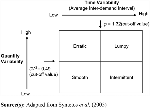
ADI measures the average number of time periods between two consecutive demands and CV2 represents the relative variability in demand quantity when demand occurs. In other words, ADI represents the intermittency of the demand pattern and CV2 represents the volatility in the quantity of demand (Syntetos and Boylan, 2005).
Much of the literature focuses on ADIs in the range of 1–10 and CV2 values of 0–2.25 (Kourentzes and Athanasopoulos, 2021; Syntetos and Boylan, 2001; Petropoulos et al., 2016). As an example, we have observed military spare part ordering data with ADIs ranging from 1 to 2.53 and CV2 values from 0.3 to 3 (McDermott, 2020; Appendix A). The ADI and CV2 values explored in this research are presented in the description of each scenario.
Demand dispersion for various intermittent demand streams (50k sample paths over 30 days horizon, average level = 3)
| Class | ADI | CV2 | E[I(t)] |
|---|---|---|---|
| Poisson | – | – | 1 |
| Smooth | 1 | 0.25 | 0.8 |
| Intermittent | 1.5 | 0.25 | 1.7 |
| 2 | 0.25 | 2.2 | |
| Erratic | 1 | 0.5 | 1.5 |
| 1 | 2 | 6.0 | |
| Lumpy | 1.5 | 0.5 | 2.5 |
| 2 | 2 | 7.5 |
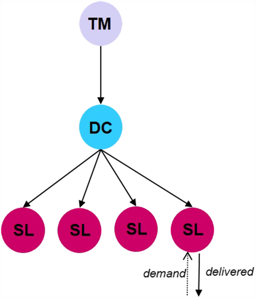
As Figure 2 illustrates, the approach uses a logistics network with different locations representing the TM source, intermediate DCs and SLs which require and consume spare parts. By modeling AM capability and locating it at various locations in the network, it is possible to assess not just AM's potential impact but the decision tradeoffs as well.
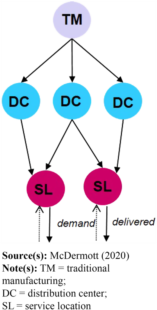
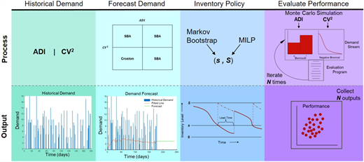
Figure 3 summarizes the methodology into a conceptual overview. First, the approach generates historical demand according to the specified characteristics (ADI, CV2), selects and constructs the appropriate demand forecast and identifies the appropriate order up to inventory policy (s, S) (Winston, 2004) using a mixed integer linear programming model where orders are placed when inventory reaches s and S denotes the order up to level. Given the appropriate inventory policy, we generate a specified number of sample paths of future demand realizations and evaluate the logistics network performance across a specified time horizon. This produces summary statistics and a performance vs cost tradeoff curve. By varying the demand characteristics or the AM configuration within the logistics network, we can assess the tradeoffs of various AM employment strategies.
3.2 Generating demand
All spare part demand data used in the evaluation of network performance is simulated. Historical demand data is generated to drive forecasts for future requirements (i.e. inventory policy) and multiple sample paths or realizations of “actual” demand are generated to evaluate the network performance via Monte Carlo simulation. The demand data is generated based on the assumption that non-zero demand arrivals follow a Bernoulli distribution and the non-zero demands a negative binomial distribution (Petropoulos et al., 2014; Kourentzes and Petropoulos, 2016). When simulating the demand, we specifically control underlying demand characteristics of ADI, CV2 and mean level of the non-zero demands.
While this assumption permits generating a wide variety of intermittent demand patterns parameterized by the ADI and CV2, it is important to note this is just a starting point as many characteristics of real-world demand are not accounted for by this schema (e.g. autocorrelation or other distributional complications). However, this captures the key features of intermittent demand described by Syntetos et al. (2005).
Regardless of the demand parameters, every realization within the same scenario has the same overall quantity of demand (±5% tolerance) over the time horizon. When simulating demand, the average demand rate is adjusted based on the ADI to ensure the overall quantity remains within the specified tolerance. Demand points with higher ADI have a higher average demand rate per period because the occurrences of demand events are less frequent across a fixed time horizon. The only difference between realizations is how demand arrives and in what quantities based on the ADI and CV2 values picked a priori. This permits performance comparisons between different demand scenarios across a fixed time horizon.
3.3 Forecasting demand
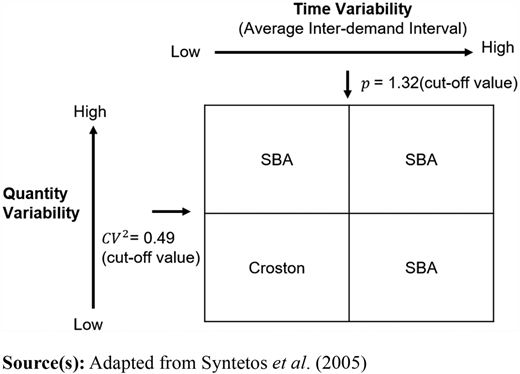
Using the simulated historical demand data for the chosen demand parameters, we forecast the future demand for the time horizon of interest. The appropriate point forecasting method for intermittent demand, either Croston's method or the Syntetos-Boylan approximation (SBA), is chosen based on the ADI and CV2 of the historical demand data, as outlined in Syntetos et al. (2005) and depicted in Figure 4. When forecasting intermittent demand using these two methods, the forecast over the time horizon is a constant value. This demand forecast is used to determine the appropriate inventory policies for locations across the network.
3.4 Determine inventory policy
Traditional methods of determining target inventory levels are appropriate where demand patterns follow a normal (Gaussian) distribution or can be approximated with a theoretical distribution. In the context of spare parts, demand is often not Normally distributed and distributional assumptions can be challenging (Syntetos et al., 2005). In order to set appropriate inventory levels for the (s(k), S(k)) policy for each of the k parts, we employ a two-stage approach.
3.4.1 Re-order point
To determine our re-order point s, we apply the “Markov Bootstrap Method” (Willemain et al., 2001, 2004, 2005). This bootstrapping method samples from the historical demand data to construct an empirical distribution of lead time demand (LTD) using the demand distribution over the replenishment lead time. The replenishment lead time is the time it takes DCs to receive requested inventory from the traditional manufacturer.
Using the empirical distribution of LTD for product k, , we observe the demand level associated with a desired customer service level, α(k) ∈ (0, 1). Based on the desired customer service level, we determine the re-order point for inventory of product k by
which is the α-quantile for product k. We arbitrarily set α = 0.75.
3.4.2 Order-up-to level
A network optimization model selects the optimal order-up-to level, annotated by S(k) in the inventory policy. The model seeks to minimize the total cost by efficiently establishing an appropriate inventory policy – unique to each DC and unique to each network configuration – based on the forecasted customer demand. Appendix B provides the mathematical formulation.
3.5 Evaluating network performance
Equipped with appropriate inventory management policies, we now evaluate the performance of the network through Monte Carlo simulation. Each network configuration is exposed to a number of sample paths of future demand requirements in the evaluation procedure. For each network configuration and each demand realization, we chronologically step through every time period over the time horizon. In each time period, there is competition for limited parts and/or resources. Inside the simulation goods and/or resources are assigned optimally using a mixed integer linear program. At the completion of the network evaluation, and for each network configuration, we have a series of data corresponding to the performance of the network for varying demand realizations. Algorithm 1 provides high level pseudo code to outline the evaluation methodology.
| Algorithm 1 Evaluation Procedure for Single Product (Monte-Carlo Simulation). | |
|---|---|
1: | Given demand parameters (ADI, CV 2 and average demand) |
2: | Generate set of demand realizations |
3: | foreach Network Configuration do |
4: | Given inventory policies (s, S) |
5: | foreach Demand Realization do |
6: | foreach t in Time Horizon do |
7: | ift = 1 then |
8: | set initial inventory |
9: | else |
10: | update inventory → inventory carried from (t – 1) and inventory replenishment |
11: | end if |
12: | Assignment sub-problem (MILP) |
→ allocate inventory and AM capacity to satisfy demandt | |
13: | ifdemandt unsatisfied then |
14: | generate backorder and update demandt+1 |
15: | end if |
16: | ifinventory remaining < re-order point (s) then |
17: | request inventory replenishment (received in accordance with replenishment lead time) |
18: | end if |
19: | end for |
20: | end for |
21: | end for |
22: | output: network configuration performance |
4. Network description
4.1 Network structure
We model the logistics network using a one-way directed graph as depicted in Figure 2. The network model used in the experimentation has three hierarchical levels and a total of six nodes. Nodes represent locations within the logistics network and arcs represent transportation routes between these nodes. Nodes include a TM plant, DCs and SLs which consume spare parts.
Within this network, we assume that AM machines can only be placed at the DCs and SLs. This implies there are 32 different combinations of ways to employ AM machines and we refer to each specific network set-up as a network configuration or design. Section 6 includes a modified network structure to analyze performance between different specific configurations.
4.2 Network characteristics and interactions
TM plants produce the set of products considered within the logistics network. We assume there is no limiting capacity or downtime in production at the manufacturing plants. This is reasonable if we assume independent production lines. Once produced, the products are transported to and stored as inventory at DCs. In response to customer demand, products are transported from the DCs to the SLs. Unused inventory is carried forward across the time horizon and inventory is replenished according to the (s, S) inventory policy. Customer demand can also be satisfied through production via AM machines that are located at DCs and/or SLs. AM production capacity will only be used to directly satisfy SL demand, it will not be used to replenish inventory stockage. The SLs generate demand at discrete daily intervals for the set of products considered. Unsatisfied demand is recorded as backorders for the following time period and continues to be carried forward until satisfied (i.e. no lost sales). All actions within the network are made in daily intervals.
Lead times in this model are comprised of production and transportation times. We assume there is no difference in lead time for the use of inventory and AM-produced parts.
4.3 Additional assumptions
AM production time is deterministic and equivalent for all part types.
The make or model of the metallic AM machine used in this research is not explicitly defined. AM production time and capacity is based on current (non-metallic) AM machine capabilities. While the current capabilities of metallic AM machines may not match their non-metallic counterparts, we believe the technology will eventually progress to the point where it is suitable for use in large-scale industrial applications.
Spare part characteristics (volume, weight and complexity) are not specified nor is the intended end-use of the part. Thus we assume that the inventory carrying cost, transportation cost, production cost and penalty cost for a backorder for any spare part is equivalent, though this is not a limitation. This assumption enables the simplification of the cost structure used in the model.
Raw materials for additive or traditional manufacturing are not considered and are always present when needed.
When there is a backorder, the end-item (machine or equipment) is not mission capable and is incurring downtime, thus there is a penalty cost associated with all shortages.
AM-produced parts are of the same quality as their traditionally manufactured counterparts. This means the failure rates of AM and TM produced parts are equivalent. This is consistent with Knofius et al. (2019), Li et al. (2017) and Abbink (2015). Without this assumption, we could expect differing demand patterns, as parts would fail at different rates depending on production source. This is a current limitation.
4.4 Cost structure
Due to limited access to data, the cost parameters used in this research are based on related literature and several assumptions. When determining the inventory policies and allocating resources, the model considers inventory carrying cost, AM machine associated costs, transportation cost and penalty costs associated with backorders. The cost values in Table 2 are adapted from studies by Abbink (2015) and Li et al. (2019) by converting to US dollars and reducing to cost per day. Logistics costs are estimated from the express shipping rates through the United Parcel Service (UPS) (Khajavi et al., 2018). Since spare part supply chains are often slow moving and low in quantity, we assume items are not shipped in bulk at discounted rates.
Cost parameters used in model
| Cost | Value | Units |
|---|---|---|
| Inventory holding cost | $ 1 | Per part per day |
| Penalty cost | $ 378 | Per part per day |
| AM-related cost | $ 121 | Per machine per day |
| Logistics cost | $ 25 | Per part |
Note(s): Adapted from the low tier cost values used in Abbink (2015) and Li et al. (2019)
The cost of production via TM and AM is highly variable and dependent on item complexity or material properties. Since we do not define spare part characteristics, it is difficult to quantify the relative cost of production in relation to each other and because of this, we assume that traditional and additive production costs are equivalent. Assuming equivalent production costs for all part types enables a clear cost structure and simplifies the experimentation.
The costs associated with purchasing, owning and operating an AM machine may include labor, materials, maintenance and depreciation. In order to keep our cost structure as clear as possible, we consolidate all these aspects into a single cost parameter: AM machine fixed cost (Li et al., 2019). This fixed cost is a function of the number of AM machines that are present in the logistics network, regardless of node location.
The purpose of our research is to explore AM-enabled configurations rather than a detailed analysis of network related costs. We rely heavily on the previous literature to derive the cost inputs for the model, though these are parameters that are easily changed. We believe the cost structure used is not only reasonable but is kept as clear and simple as possible while achieving our research objectives. While this research relies on the “low” cost data proposed by Abbink (2015), initial experimentation shows the model results to be relatively insensitive to changing cost data (moderate and high) (McDermott, 2020; Appendix D).
5. Performance tradeoffs for AM-enabled network configurations
5.1 Scenario description
This section applies the methodology and assumptions to the network presented in Figure 2 to assess if intermittent demand properties affect network performance. The objective is to capture the performance, in terms of cost and backorders, of all possible network configurations and understand tradeoffs associated with each. Doing so enables decision-makers to analyze the alternatives of where and how to allocate their AM capability to best support their needs. In this specific scenario we assess network performance based on the demand of three spare parts with lumpy demand patterns using demand parameters of ADI = 1.48, CV2 = 0.73 and a mean non-zero demand value of 3. Demand streams are generated at each of the SLs. AM production capacity per machine per period is 1 unit and no more than one machine can be placed at each node. Using Monte Carlo simulation, we evaluate each network configuration for 50 realizations of demand over a 60 days’ time horizon. The time it takes to produce and transport product from the TM to the DCs is 7 time periods. The lead time from the DCs to the SLs is 2 days.
5.2 Tradeoff analysis
Enumerating all possible ways to include AM in the network, the 32 configurations from Figure 5 demonstrate the potential for increased AM capacity in the spare parts supply chain to improve performance (reduce backorders) while increasing total costs. Adding AM to the network also results in reduced variability in the performance as measured by total backorders. Removing the fixed costs associated with AM machines, we observe purely the operating costs of a network (see Figure 6). Heavily AM-enabled configurations are largely more cost efficient as AM capacity replaces on-hand inventory, thereby reducing inventory carrying costs and permitting AM machines to be located closer to the end-user which reduces the transportation and logistics costs. Figure 7 averages the performance outputs of Figure 5 for a more clear representation of the tradeoffs per configuration.
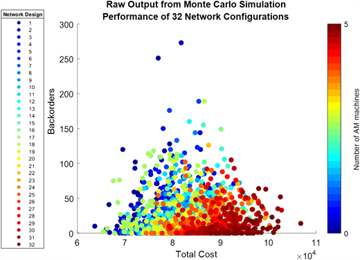
(Color online) Monte Carlo simulation raw output results. Data points are grouped by each of the 32 network configurations
(Color online) Monte Carlo simulation raw output results. Data points are grouped by each of the 32 network configurations
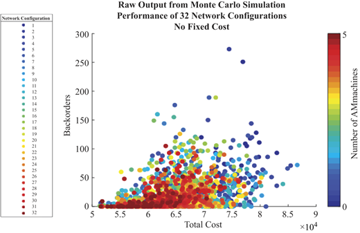
(Color online) Monte Carlo simulation raw output results with AM fixed costs removed. Data points are grouped by each of the 32 network configurations
(Color online) Monte Carlo simulation raw output results with AM fixed costs removed. Data points are grouped by each of the 32 network configurations
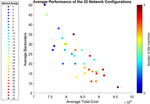
(Color online) Performance results from Monte Carlo simulation. Results condensed by averaging the backorders and total cost. Each network configuration is represented by a single point on the graph
(Color online) Performance results from Monte Carlo simulation. Results condensed by averaging the backorders and total cost. Each network configuration is represented by a single point on the graph
However, Figure 8 shows that the associated tradeoffs between performance and cost are highly dependent on characteristics of the spare part demand. Here we observe the relative value of AM addition to the supply chain when the underlying demand characteristics differ. Network performance for all 32 configurations is evaluated under four different demand scenarios, one for each demand classification and then compared. The value of employing AM machines inside a network can be surmised from the general slope of a line fitted to the performance of each demand scenario because generally speaking, as we move from left to right in Figure 8, we add AM machines to the network. On a marginal basis, employing AM in a network servicing lumpy demand makes roughly 11 times the impact as compared to employing AM in a network servicing smooth demand.
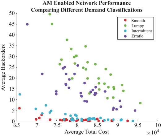
(Color online) Average network performance organized by underlying classification of demand. Demand class defined by parameters: Smooth: ADI = 1.16, CV2 = 0.24; Erratic: ADI = 1.16, CV2 = 0.73; Intermittent: ADI = 1.48, CV2 = 0.24; Lumpy: ADI = 1.48, CV2 = 0.73. Average non-zero demand value of 3 for all scenarios
(Color online) Average network performance organized by underlying classification of demand. Demand class defined by parameters: Smooth: ADI = 1.16, CV2 = 0.24; Erratic: ADI = 1.16, CV2 = 0.73; Intermittent: ADI = 1.48, CV2 = 0.24; Lumpy: ADI = 1.48, CV2 = 0.73. Average non-zero demand value of 3 for all scenarios
The forecastability or stability of demand is a key factor when determining the value of AM incorporation in a spare part supply chain with inventory holdings. AM machines serve as a stop gap or supplement to the current logistics network, but since smooth demand is easy to forecast (leading to effective inventory control), there is little need for such contingency AM capacity and machines sit idle. However, networks servicing lumpy demand greatly benefit from the addition of AM machines to the network. Here, AM machine capacity is used more efficiently as there are more frequent inventory stock outs due to poorer performance of the inventory policy.
This is not to say that AM is not useful to support smooth demand as AM can still serve as a stop-gap to address temporary shortages and can be a capability for the decision-maker to employ when needed. For example, in some military applications this capability would be a great asset to the commander and it may be well worth the expense to have such an asset on reserve, even if idle, as a risk mitigation strategy.
A modified version of this network with more complex nodal interactions is also explored (i.e. the capability to expedite the production and transport of parts and lateral transfer of inventory between DCs). The subjective nature of the capacities associated with these additional capabilities requires more research as to an appropriate range of values. The model details and preliminary results for this network with more complex nodal interaction can be found in McDermott (2020; Appendix B).
6. Performance comparison for various demand patterns
6.1 Scenario description
Understanding demand characteristics plays a significant role in AM-enabled network performance. To capture these impacts, we explore the performance of three different network configurations – centralized, distributed and traditional (no AM) – with different demand characteristics. Our objective is to identify the demand characteristics where the performance (in terms of backorders) of the centralized configuration dominates the distributed and vice versa.
For all remaining studies, the logistics network pictured in Figure 9 is used and this modification is made for purposes of clarity and simplification. This network is comprised of a traditional manufacturer, a DC and four different SLs. In order to explore the entire state-space of appropriate values, we evaluate 500 realizations of demand associated with a single product for all combinations of ADI values from 1 to 5 and CV2 values of 0, 0.25–4.85 with increments of 0.2. Here, a demand stream is generated from the perspective of the DC and then the demand is randomly assigned to the SLs. This method ensures the demand, from the perspective of the DC, has the exact characteristics that we desire. With this method, we essentially remove the effects of aggregation on the demand characteristics. AM machine production capacity is set to 4 units per period and the average demand is 3. All other input parameters remain unchanged unless noted.
Network used to evaluate centralized and distributed configurations for all demand characteristics
Network used to evaluate centralized and distributed configurations for all demand characteristics
This model employs what is referred to as a “reactive” inventory policy. For every change in underlying demand pattern (ADI or CV2 combination) the model updates the optimal inventory policy. This scenario is representative of how an organization may seek to efficiently implement AM capabilities, assuming the organization is aware of the characteristics of their demand and is able to detect demand changes, though in our model the ADI and CV2 will be constant across the specified time horizon.
6.2 Performance comparison: results
From a macro perspective, Figure 10 displays the best performing network configuration across the entire ADI and CV2 state-space of interest. Recall that regardless of the demand parameters, every scenario is exposed to the same overall quantity of demand (±5% tolerance) over the time horizon. The only difference between scenarios is the underlying demand patterns of how and when demand arrives. For each point in Figure 10, there are three configurations evaluated, each with 500 sample paths, to find the best performance. The label “No AM/Dist/Cent” indicates that the Traditional (no AM) configuration performed as well as the distributed and centralized configurations. Similarly, the “Dist/Cent” label identifies where there was no performance difference (±3%) between the distributed and centralized configurations.
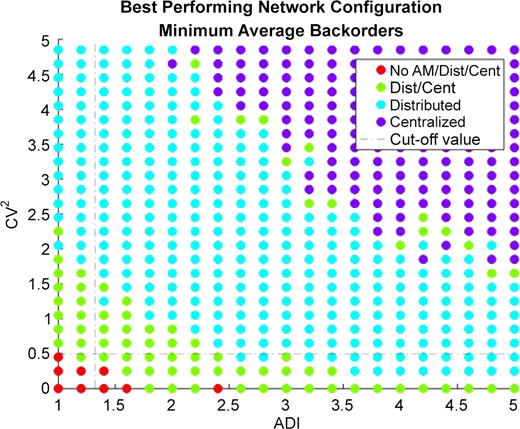
(Color online) The best performing network configuration, in terms of lowest average backorders, across all CV2 and ADI value combinations. (Parameters: reactive inventory policy, AM capacity: 4, Average demand: 3, Demand realizations: 500, Products: 1.)
(Color online) The best performing network configuration, in terms of lowest average backorders, across all CV2 and ADI value combinations. (Parameters: reactive inventory policy, AM capacity: 4, Average demand: 3, Demand realizations: 500, Products: 1.)
The centralized configuration dominates performance in the high ADI and CV2 value range. Here the pooling of demand and AM capacity upstream in the supply chain enable the centralized configuration to address the sporadic arrival of lumpy quantities of demand. Such arrivals of demand would either exceed the AM production capacity of the distributed configuration or AM capacity would sit idle for extended periods.
Lower ADI and CV2 value combinations favor the distributed network configuration. Lower values indicate a more stable demand pattern in terms of arrival rate and quantity and here the distributed AM machines are using their production capacity more efficiently. Table 4 provides the summary statistics for several ADI, CV2 values.
Summary statistics of select ADI, CV2 values for scenario with parameters: AM machine capacity: 4, Average demand: 3, Realizations: 500, Products: 1
| CV2 | ADI | Configuration | Min inventory (s) | Max inventory (S) | Mean backorders | Half-width (α = 0.05) | Standard deviation | % Demand AM produced |
|---|---|---|---|---|---|---|---|---|
| 0.25 | 1.2 | Traditional | 33 | 65 | 0.17 | 0.09 | 1.07 | 0.00 |
| Distributed | 33 | 34 | 0.00 | 0.00 | 0.00 | 100 | ||
| Centralized | 33 | 34 | 0.00 | 0.00 | 0.00 | 0.00 | ||
| 0.25 | 3.4 | Traditional | 34 | 58 | 22.60 | 2.57 | 29.26 | 0.00 |
| Distributed | 34 | 36 | 0.00 | 0.00 | 0.00 | 89 | ||
| Centralized | 34 | 35 | 0.36 | 0.14 | 1.57 | 8 | ||
| 3.45 | 1.2 | Traditional | 38 | 62 | 37.41 | 4.62 | 52.72 | 0.00 |
| Distributed | 38 | 40 | 0.81 | 0.37 | 4.18 | 84 | ||
| Centralized | 38 | 39 | 3.07 | 0.76 | 8.62 | 8 | ||
| 3.45 | 3.4 | Traditional | 25 | 31 | 646.04 | 36.47 | 416.03 | 0.00 |
| Distributed | 25 | 28 | 59.26 | 6.21 | 70.84 | 70 | ||
| Centralized | 25 | 26 | 56.24 | 5.21 | 59.40 | 38 | ||
| 4.85 | 4.8 | Traditional | 19 | 37 | 947.11 | 499.26 | 43.76 | 0.00 |
| Distributed | 19 | 22 | 166.55 | 120.84 | 10.59 | 71 | ||
| Centralized | 19 | 20 | 150.93 | 111.80 | 9.80 | 55 |
These tradeoffs between configurations are clearly displayed in Figure 11 when we look at the percent of the total demand that is satisfied via AM-produced parts. The graph presents results for all ADI values for a fixed CV2 value of 2.65 (a single row from Figure 10). Looking at the centralized configuration, as the demand becomes more irregular, the upstream pooling becomes more apparent evidenced by the increased AM production. Conversely, the increasingly irregular and lumpy arrivals of demand overwhelm and/or leave AM capacity in the distributed configuration idle, as indicated by a decrease in production rate.
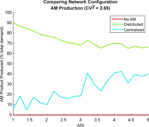
(Color online) Comparison of the amount of product produced via AM (in terms of percent of total demand) between network configurations
(Color online) Comparison of the amount of product produced via AM (in terms of percent of total demand) between network configurations
The performance effects of pooling are clearly displayed in Figure 12. As ADI values increase, the centralized configuration outperforms the distributed configuration. The magnitude of the performance gap also grows larger as ADI increases, largely due to the pooling effect. As the demand becomes more irregular and lumpy, the AM capacity in the centralized configuration is used much more efficiently and therefore outperforms the distributed configuration. The pooling effect and more specifically, the percent of total demand satisfied via AM production can be observed across the entire state space in Figures A1 and A2 in Appendix C. As expected, the addition of AM capacity into the network results in the dominance in performance of the AM-enabled configurations. Additionally, the AM capacity serves to reduce the variance in performance as compared to the traditional (no AM) scenario.
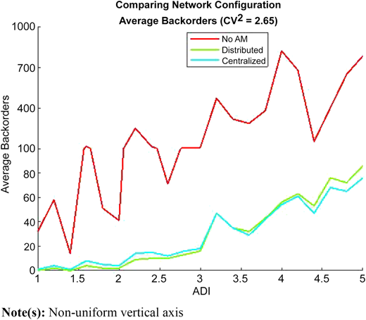
(Color online) Performance comparison of network configurations with CV2 = 2.65 for all ADI values
(Color online) Performance comparison of network configurations with CV2 = 2.65 for all ADI values
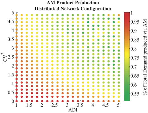
(Color online) Percentage of total demand that was produced via AM in the distributed configuration. (Parameters: reactive inventory policy, AM capacity: 4, Average demand: 3, Demand realizations: 500, Products: 1.)
(Color online) Percentage of total demand that was produced via AM in the distributed configuration. (Parameters: reactive inventory policy, AM capacity: 4, Average demand: 3, Demand realizations: 500, Products: 1.)
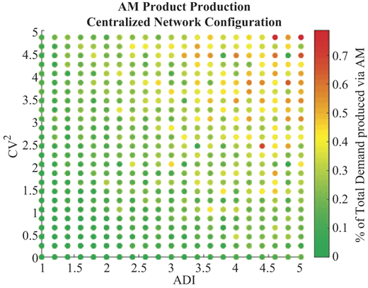
(Color online) Percentage of total demand that was produced via AM in the centralized configuration. (Parameters: reactive inventory policy, AM capacity: 4, Average demand: 3, Demand realizations: 500, Products: 1.)
(Color online) Percentage of total demand that was produced via AM in the centralized configuration. (Parameters: reactive inventory policy, AM capacity: 4, Average demand: 3, Demand realizations: 500, Products: 1.)
Figure 10 indicates the best performing network configuration on average but conveys no information as to how much better performing a network configuration is or if the results are even practically significant. The high time variability (ADI) and quantity variability (CV2) require extraordinary computational effort to see the centralized configuration dominate in a practically significant sense. Exploratory studies have confirmed for higher ADI and CV2 value combinations, the confidence intervals indeed diverge with additional samples. The dominance observed is consistent with the results comparing the mean values and more information can be found in McDermott (2020). Table 3 summarizes the percent gap in configuration performance for the different configuration regions of dominance.
Average percent gap for average backorders using decision boundaries applied to Figure 10
| Best performing network configuration | Mean gap (%) |
|---|---|
| No AM/Dist/Cent | 0.0 |
| Dist/Cent | 0.0 |
| Distributed | 39.0 |
| Centralized | −11.0 |
Note(s): Positive numbers imply the distributed configuration has fewer backorders than the centralized configuration. Decision boundaries obtained using support vector machines with nonlinear kernels (James et al., 2013). (Parameters: same as Figure 10)
The results presented here reflect the efficient application of AM capacity in conjunction with an appropriate inventory management policy. If we change our assumptions to reflect a firm that does not appropriately understand their demand, or cannot react to changing demand patterns, we can explore the upper bound on the benefits AM addition can provide. The interested reader can observe the modeling process and results from a “fixed” inventory scenario in McDermott (2020, Appendix C).
Sensitivity analysis confirms the results are robust to length of time horizon and the number of demand sample paths, though as expected, additional sample paths increase the boundary fidelity between the centralized and distributed configurations in the ADI, CV2 space. The interested reader can refer to McDermott (2020, Appendix D) for extensive sensitivity analysis results.
7. Relationship between demand volume and AM capacity
For broader generalizations of AM employment strategies, we explore scenarios with low or high AM production capacity facing low or high demand volume. The values used in this sensitivity analysis are based on highly intermittent demand datasets found in research by Petropoulos et al. (2016) and Willemain et al. (2004). The values used are: average demand size (low = 1, moderate = 3, high = 8) and AM capacity per machine per period (low = 1, high = 4).
For a given AM capacity, comparing performance for increasing demand volumes highlights the tradeoffs between centralized and distributed configurations. As demand volume increases, and more specifically as the relative gap between demand volume and AM production capacity increases, the benefits of pooling become more apparent through the increasing regional dominance of the centralized configuration as seen in Figures 13–15.
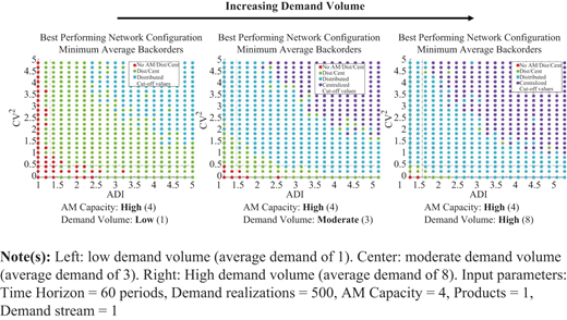
(Color online) Comparison of network configuration performance for a fixed AM machine capacity of 4 parts per period and increasing demand volume
(Color online) Comparison of network configuration performance for a fixed AM machine capacity of 4 parts per period and increasing demand volume
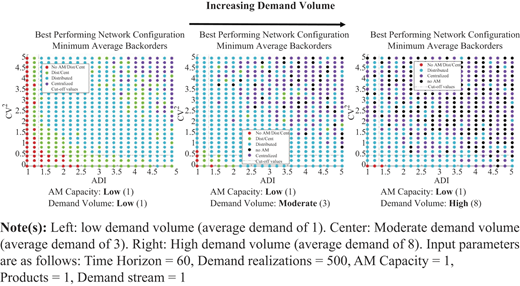
(Color online) Comparison of network configuration performance for a fixed AM machine capacity of 1 part per period and increasing demand volume
(Color online) Comparison of network configuration performance for a fixed AM machine capacity of 1 part per period and increasing demand volume
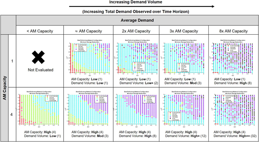
(Color online) Compares network performance and the relationship between AM production capacity and total demand volume. Explores AM production capacity of 1 and 4 parts per period for increasing total demand observed over the time horizon. Annotated below each chart is the AM machine production capacity and the average demand
(Color online) Compares network performance and the relationship between AM production capacity and total demand volume. Explores AM production capacity of 1 and 4 parts per period for increasing total demand observed over the time horizon. Annotated below each chart is the AM machine production capacity and the average demand
The results (Figure 13) show that when AM capacity is high and demand volume is low, the distributed configuration dominates the entire state-space as this distributed AM capacity is not often overwhelmed. When demand volume is high, the distributed AM capacity is overwhelmed in the upper ADI, CV2 value ranges and the benefits of pooling in the centralized configuration become apparent. The greater the disparity between average demand and AM machine capacity, the “earlier” the benefits of pooling are realized, as indicated by the dominance of the centralized configuration creeping into lower value ranges when comparing results of Figure 13.
The same general conclusions and interactions hold true when AM capacity is low (Figure 14). We do however, see an interesting tradeoff between the centralized configuration and the traditional (no AM) configuration as demand volume increases. This is a result of the interaction between the relatively small amount of pooled AM capacity upstream and the traditional (no AM) configuration holding large quantities of inventory to address the high levels of demand. McDermott (2020, pp. 76–80) shows that by removing this apparent tradeoff and solely comparing the AM-enabled configurations we see clear delineations of regional dominance. We confirm that in the higher ADI and CV2 value range, the centralized configuration performs best due to the pooling effects previously highlighted in this research.
8. Conclusion
This paper expands upon previous research in the field of AM employment configurations in two key ways. Within the framework of the demand classification scheme proposed by Syntetos et al. (2005), this paper provides a demand-focused modeling approach to study the impact of AM addition to a supply chain and, to the best of our knowledge, is the first paper to map AM-configuration performance tradeoffs to intermittent demand properties common to spare parts supply chains. Additionally, this paper explores a performance tradeoff curve for all possible AM-enabled network configurations. The methodology employed in this research is based upon how an organization would seek to conduct an analysis of alternatives before employing AM capability within their supply chain. Through the simulation of historical demand data, forecasting of future demand requirements and determination of appropriate inventory policies, we compare performance of network configurations and explore tradeoffs associated with each.
This research assesses the preferred AM-enabled supply chain configuration for varying levels of intermittent demand patterns and AM production capacity. We demonstrate that variation in demand patterns alone directly affects the preferred network configuration and highlight the dominance of the centralized configuration in the high ADI, CV2 value range due to pooling of both AM capacity and demand upstream in the supply chain. The tradeoffs between the centralized and distributed configuration are quite clear in our results. Further understanding of the tradeoffs between the distinctly opposite allocation strategies is brought about through sensitivity analysis of the relationship between demand volume and relative AM production capacity. The results show that the relationship between the demand volume and relative AM production capacity also affects the network configuration performance.
8.1 Future work
Future work should include detailed modeling of AM technology parameters to include build failure probability, build chamber capacity, part size and complexity, machine costs and post-processing requirements. While we would expect an increase in build failure probability to favor the centralized configuration these other modeling parameters would only bring greater model fidelity for a specific spare part supply chain.
A natural extension of this work is to explore multi-product scenarios with heterogeneous demand patterns. Additionally, exploring a more complex, multi-echelon network structure with additional nodal interactions should be considered. These aspects will bring further realism and value for a number of applications.
Interesting extensions of this work include the application of AM to disaster relief or military operations. First would be to understand how AM machines can enable or support a rapidly responsive supply chain. Such scenarios model disaster relief efforts or response to the COVID-19 pandemic, where product demand quickly and temporarily surges. Also, another source of variability would be the availability of nodes in the network.
Military logistics networks, especially those forward deployed, have several unique characteristics not seen in conventional supply chains. Military logistics networks are at risk of disruption from adversaries and it would be interesting to explore how AM insertion supports the dis-aggregation of the network. A decentralized network configuration may increase the robustness of the network and reduce the impact of disruptive events.
This work was supported, in part, by a grant from the U.S. Army Research Office (grant# W911NF1910055). A special thanks to Smart Software, Inc. for sharing the “Markov Bootstrap” with us. The authors are also indebted to Marc Robbins from RAND for providing the Operation Iraqi Freedom spare part orders dataset which helped us choose ADI and CV2 values for our study. The authors are grateful for the helpful suggestions from H.L. Jones who braved this paper in draft form. This paper also benefited from constructive comments from the editor and two reviewers that improved both the content and presentation.
Disclaimer: The views expressed in this paper are those of the authors and do not reflect the official policy or position of the United States Army, the Department of Defense, or the United States Government.
References
Appendix
| Sets | |
|---|---|
N | network locations |
N̄ | set of nodes upstream of node n |
| set of nodes downstream of node n |
P⊂ N | traditional manufacturing plants |
DC⊂ N | distribution centers |
SL⊂ N | service locations |
G | set of spare parts |
T | time horizon |
Index Use | |
i∈ N | node locations |
i'∈ N̄ | index for locations upstream of i that supply node i |
| index for locations downstream of i that are serviced by i |
t∈ T | time index |
g∈ G | index for spare parts |
Decision Variables | |
TMproduceitg | quantity of part g traditionally produced in period t at location i ∈ P |
AMproduceitg | quantity of part g produced with AM in period t at location i∈ {DC, SL} |
| flow of part g transported from location i to i" in period t |
invitg | quantity of part g carried as inventory at location i ∈ DC from period t – 1 to t |
backorderitg | quantity of unsatisfied demand of part g at location i∈ SL from period t – 1 to t |
Given Data | |
| cost to traditionally produce part g at location i∈ P in period t |
| cost to produce part g with AM at location i ∈ {DC, SL} in period t |
| cost to transport part g from location i to i" in period t |
| cost of carrying inventory of part g at location i ∈ {DC, SL} from period t – 1 to t |
| penalty cost for unsatisfied demand of part g at location i ∈ SL in period t |
demanditg | demand for part g at location i ∈ SL in period t |
AMcapacityitg | AM production capacity for part g at location i ∈ {DC, SL} in period t |
| initial inventory of part g at location i ∈ DC |
| lead time between locations i' and i for part g |
Auxiliary Variables | |
MinPolicyig | inventory level for part g at which a re-order will be placed at location i ∈ DC |
MaxPolicyig | inventory ‘order up to’ level for part g at location i ∈ DC |
delivereditg | quantity of part g delivered to location i ∈ SL to satisfy demand in time period t |
reorderQTYitg | amount of part g ordered at location i ∈ DC in time period t |
Pitg | indicator if reorder required for part g at location i ∈ DC in time period t |
eitg | AM production indicator for part g at location i ∈ {DC, SL} in time period t |
M | large number |
p, e≥ 0 and binary | |
all others non-negative and integer | |
A. Demand dispersion
For an stochastic process counting the number of events (arrivals) by time t, the index of dispersion (for counts) is
It is well known that if is a Poisson process, stationary or otherwise, then I(t) = 1 for all t. Consequently, the process is underdispersed if I(t) < 1 and overdispersed if I(t) > 1. Table A1 demonstrates the Poisson process assumption may not be appropriate for some spare parts with intermittent demand. For intermittent demand with constant ADI and CV2 parameters, the resulting dispersion will also be a constant.
B. Selecting the inventory policy
Summary statistics of several ADI, CV2 values for scenario with parameters: AM machine capacity: 1, Average demand: 3, Realizations: 500, Products: 1
| CV2 | ADI | Configuration | Min inventory (s) | Max inventory (S) | Mean backorders | Half-width (α = 0.05) | Standard deviation | % Demand AM produced |
|---|---|---|---|---|---|---|---|---|
| 0.25 | 1.2 | Traditional | 29 | 53 | 0.78 | 2.29 | 0.20 | 0.00 |
| Distributed | 29 | 43 | 0.00 | 0.00 | 0.00 | 67 | ||
| Centralized | 29 | 30 | 0.07 | 0.57 | 0.05 | 1 | ||
| 0.25 | 3.4 | Traditional | 29 | 53 | 48.80 | 55.20 | 4.84 | 0.00 |
| Distributed | 29 | 35 | 7.20 | 13.99 | 1.23 | 36 | ||
| Centralized | 29 | 30 | 21.79 | 24.26 | 2.13 | 10 | ||
| 3.45 | 1.2 | Traditional | 29 | 41 | 112.54 | 111.62 | 9.78 | 0.00 |
| Distributed | 29 | 37 | 32.50 | 52.13 | 4.57 | 49 | ||
| Centralized | 29 | 30 | 47.04 | 56.84 | 4.98 | 12 | ||
| 3.45 | 3.4 | Traditional | 32 | 35 | 416.02 | 331.15 | 29.03 | 0.00 |
| Distributed | 32 | 37 | 187.81 | 173.82 | 15.24 | 32 | ||
| Centralized | 32 | 33 | 178.77 | 162.76 | 14.27 | 20 | ||
| 4.85 | 4.8 | Traditional | 25 | 34 | 891.44 | 532.28 | 46.66 | 0.00 |
| Distributed | 25 | 31 | 478.81 | 300.01 | 26.30 | 34 | ||
| Centralized | 25 | 26 | 473.89 | 298.08 | 26.13 | 32 |
B.1. Model
Objective function
s.t.
B.2. Model discussion
Indexing. The nodes that comprise the logistics network include the TM plant P, distribution centers DC and service locations SL. For each node, i, there exist a set of “upstream” nodes, i′ indexed by , that supply node i. There also exists a set of downstream nodes i″ index by , that can be supplied by node i. Valid routes within the network are represented by all i′,i and i,i″ pairs.
Objective function. The objective (3) seeks to minimize the total cost by selecting the appropriate inventory policy (s, S) that ensures the efficient allocation of products to meet the forecasted demand requirements.
Flow balance constraints. The flow balance for all network nodes can be, in general terms, characterized by the inventory carried from time t to t + 1 and the transportation of products in terms of inflow from upstream nodes and outflow to downstream nodes. Additional considerations need to be taken for DC or SL nodes when additive manufacturing capability is available to ensure flow balance.
Constraint (4) represents the flow balance for TM plants in terms of the amount of product g produced at and transported from TM plant i to the set of downstream nodes i″ in time period t.
Constraint (5) represents the flow balance for DCs in terms of the inventory carried between periods t to t+1, the amount of product g transported in via route i′,i and out via route i,i″. Lagi′i represents the lag time along route i′,i for product to go from TM plant i′ to DC i. The lag time is an integer value in terms of days.
Constraint (6) represents the flow balance for SLs. It differs from DC flow balance in that we introduce the delivereditg variable to account for the delivery of product from the SL to the end user who will consume the product. Here we view the SL as co-located with the end user and therefore, there is no time delay in receipt of product from a DC, to delivery of the product to the end user. It is simply an “administrative” variable that enabled the consolidation of all the product received at a SL and will be used in the backorder constraint.
Constraint (7) represents the flow balance for backorders; if there is unsatisfied demand at the end of a time period, then a backorder is carried forward in the time horizon until demand is met. There are no lost sales.
Inventory replenishment constraints. Constraints (9–12) comprise the logic for the replenishment of inventory stock. If the inventory carried to the following time period is less than the re-order point, then binary variable p is activated indicating a inventory replenishment is required. In order to determine the appropriate order quantity, Constraint (13) is used. Of note, this constraint is nonlinear and the linear transformation of it is represented by Constraints (18–21) below. This constraint reads, if an inventory replenishment is required, then the reorder quantity is the difference between the “order-up-to” point and current inventory. Constraint (14) ensures re-ordered inventory is transported to the proper DC.
AM production constraints. Constraints (16–17) represent AM machine production capacity and restriction (i.e. a single machine only produce a single product type at a time).
C. Supplemental results
Figures A1 and A2 represent the amount of AM-produced product for the distributed and centralized configurations. Note the scale on the Figures if conducting comparison.
