The purpose of this paper is to improve the air movement operations planning heuristic in the literature to generate better solutions in a shorter time period.
Through a rigorous design of experiments (DOEs), we make significant heuristic improvements by evaluating alternative modular methodologies and tuning heuristic parameters for two scenarios. This includes a new approach to considering refueling operations.
We find the fine-tuned heuristic averages a 33% objective improvement and 70% reduction in computation time over the heuristic with original parameters for one of the scenarios. Additionally, we analyze the heuristic's quality of solution over time.
Further analysis is required to generalize heuristic settings, which would require significant access to operational data or a portfolio of scenarios of interest.
Tuned heuristic parameters reduce the computation time from hours to minutes. This also makes it practically feasible to adjust parameters in the objective function to generate multiple courses of action (COAs) for a given instance.
This research provides novel vehicle assignment and routing heuristic improvement alternatives and demonstrates a DOEs-based heuristic tuning procedure.
1. Background
US Army units solicit helicopter support from Army Aviation units using an Air Mission Request (AMR) process (Department of the Army [DA], 2020a) to support air movement operations which move personnel, supplies, and equipment throughout an area of operations (Department of the Army [DA], 2020b). The unit requesting support routes the AMR through their chain of command where higher echelons conduct quality control and consolidates the requests for onward submittal to the next echelon. At the brigade level, the brigade aviation element (BAE) provides aviation subject matter expertise for filtering and prioritizing the AMRs to best employ helicopter assets. The BAE submits the final AMRs to the next headquarters, usually a division. The division tasks the AMRs to the aviation unit for execution. Standard processing times from the BAE’s receipt of the tasking to the planned air movement is 96 h, though dynamic requirements often involve requests submitted within 24 h of the desired movement.
The aviation unit tasks the AMRs to the appropriate subordinate aviation battalions and/or task forces based on mission type, required equipment, aircraft needed, and other factors. These aviation battalions must task each AMR to an aircraft team and generate routes for the aircraft team to complete all assigned AMRs and associated requirements. No later than 12 h prior to the desired time of air movement, the aviation unit publishes a daily air movement table to convey the results of the planning process back to the unit requesting aviation support.
Aviation mission planners have 12 h (although often less) to task and route aircraft teams to support the AMRs based on AMR priority levels, locations, number of personnel and pickup/drop-off time windows. According to a current general support aviation battalion commander, the current process can take a team of planners over five hours to generate a plan for a single day (Espinoza, 2022). Nelson et al. (2023a) introduce two models to task air mission requests (AMRs) to rotary wing aircraft teams and generate the required routes in order to minimize unsupported AMRs by priority level, number of helicopter teams used by utilization penalty and total flight hours. A mixed integer linear program (MILP) is developed which generates optimal solutions but proves intractable for application-sized instances with 30–100 AMRs. A heuristic approach is developed which generates feasible solutions within a tactically useful time, but the authors note future work to potentially improve the heuristic. In this paper we investigate methodologies to improve the aviation air movement operations planning heuristic in order to generate superior solutions in less time. We make improvements by incorporating several alternative modular methodologies and optimizing heuristic parameters. The findings result from data collected during a rigorous design of experiments (DOE). This paper demonstrates its value in its final presentation of solution quality and time for various application-sized problems and compares the performance to Nelson et al. (2023a).
2. Literature review
2.1 Related literature
This research is not the first to envision new systems or tools to improve military decision-making, planning and dynamic re-planning, or resource-allocation with automation (McQueary et al., 2005; Rogers et al., 2018; Schwartz et al., 2019; McConnell et al., 2021) including aviation support use cases (Ghigliotti et al., 2022; Nelson et al., 2022). Much of the military aviation planning literature centers on flight and maintenance planning (FMP) to identify which aircraft to fly and which aircraft should enter maintenance over a given planning horizon with the stated objective to maximize fleet availability and meet both flight and maintenance requirements (Pippin, 1998; Kozanidis et al., 2010; Marlow and Dell, 2017). MILP approaches are common (Pippin, 1998; Kozanidis et al., 2014; Verhoeff et al., 2015; Marlow and Dell, 2017; Verhoeff and Verhagen, 2023) though some use heuristics and metaheuristics (Steiner, 2006; Winata, 2011; Kozanidis et al., 2014; Balakrishnan et al., 2021), simulation (Marlow et al., 2019), or approximate dynamic programming (Powell, 2014). Notably in our problem, the planners are not concerned with the maintenance or future demand planning.
2.2 Similar work
The most closely related literature is the dial-a-ride problem (DARP) (Ho et al., 2018b; Nasri et al., 2021) and military studies assigning assets to missions while considering the associated operational capacities, demands, routes, time windows, etc. These studies examine heterogeneous mobility rotary-wing units (Kim and Kim, 2011; Mogensen, 2014; Nelson et al., 2023a; Nelson, 2023), fixed-wing fleets (Brown et al., 2013), amphibious ready groups with multiple ship types, marines and different aircraft (Yakıcı et al., 2018), and matching air assets to tactical air requests (Noble et al., 2015). Common approaches in these problems include MILP models (Brown et al., 2013; Yakıcı et al., 2018; Nelson et al., 2023a), heuristics (Kim and Kim, 2011; Mogensen, 2014; Yakıcı et al., 2018; Nelson et al., 2023a), and metaheuristics (Cordeau and Laporte, 2003; Noble et al., 2015; de Alvarenga Rosa et al., 2016; Ho et al., 2018a); mixed approaches are common.
In a closely related study, Kim and Kim (2011) also focus on the air movement operations problem, but they minimize the time by which all missions are completed and assume aircraft have the fuel capacity to handle all assigned missions for the day. Their experimentation includes problem instances of 5–20 aircraft and 5–25 missions per day; however, their problem instances use randomly generated mission start/end points using the uniform distribution in a square plane. Brown et al. (2013) address a fixed-wing DARP problem over both single day and seven day time horizons for Iraq and Afghanistan-based scenarios, assuming that airplanes may refuel at any landing node.
The MILP model in Nelson et al. (2023a) solves the US Army aviation air movement operations planning problem (Nelson et al., 2022) by formulating it as a DARP where refueling is available at some but not all helicopter landing zones (HLZs). The paper’s research draws heavily on DARP research from Cordeau and Laporte (2007), Ho et al. (2018b), and Nasri et al. (2021). The MILP includes additional features such as capacitated helicopter routing and multi-node refueling (de Alvarenga Rosa et al., 2016; Sundar and Rathinam, 2012; Sundar et al., 2016). However, Nelson et al. (2023a) show that optimal solutions cannot be found in a reasonable amount of time for more than around three aircraft teams and 10 AMRs. The air movement operations planning heuristic is an adaptation of the insertion algorithm for the single vehicle DARP (Häme, 2011) into a multi-helicopter team heuristic to find quality feasible solutions to application-sized instances of the problem with 10 aircraft teams and 90–100 AMRs.
The purpose of this research is to improve the air movement operations planning heuristic solution quality and computation time. In this paper, we demonstrate improvement through parameter tuning. Research in parameter tuning involves numerous methods, including teacher–learner optimizing algorithms (Yang et al., 2018; Rao and Kalyankar, 2013), robust observer approaches (Beelen et al., 2020), and data analysis parameter approximation techniques (Wang et al., 2020).
Similar to this paper’s methodology, there is ample research using DOE to tune model parameters. Lujan-Moreno et al. (2018) use DOE to screen the most important machine learning hyperparameters followed by a response surface methodology to fine-tune the hyperparameters. Shankar et al. (2022) use DOE and response surface design to ascertain the key synthesis parameters and develop synthesized O-doped boron nitride models. O’Connor and English (2021) demonstrate a systematic factorial-design DOE to estimate optimal parameters of empirical water models. We use a methodology adapted from Gunawan et al. (2011) in creating a DOE approach to fine-tune algorithm parameters.
3. Air movement operations planning heuristic
3.1 Fixed time heuristic
Nelson et al. (2023a) employ a heuristic that terminates when no improvement is made to the objective in subsequent improvement cycles, which then returns the best solution found. To compare performance for varying heuristic settings, Figure 1 presents the heuristic modified to run for a fixed amount of time.
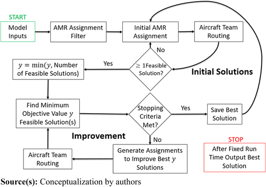
Similar to the heuristic in Nelson et al. (2023a), the fixed time heuristic starts with loading model inputs and determining which helicopter teams can support each AMR through the AMR assignment filter. The set of individually feasible AMRs per aircraft team is then sent to the initial AMR assignment module where it generates a set number of random assignments. In the original heuristic, the initial AMR assignment module randomly assigns AMRs to any helicopter team in the feasible AMR set. In this paper, we introduce a parameter to control the percentage of initial assignments that allow for unsupported AMRs or assignments to high-cost helicopter teams. High-cost aircraft teams are defined by the user when evaluating each aircraft team’s utilization penalty, β. This parameter is further discussed in Section 4.2. The set of initial assignments then goes through the aircraft team routing algorithm adapted from the single vehicle DARP adaptive insertion algorithm (Häme, 2011). This paper introduces an additional aircraft team routing algorithm that has the capability of inserting refueling stops at HLZs that do not have an associated AMR pickup or drop-off. Section 4.3 goes into further detail regarding the differences in the two aircraft team routing algorithms considered. Additionally, Section 4.4 evaluates the performance of the feasible route limit objectives described in Nelson et al. (2023a).
For each initial assignment, the aircraft team routing algorithm outputs either a feasible routing for each aircraft team or determines that the AMR assignment is infeasible. If there are no feasible assignments, the heuristic returns to the initial AMR assignment module and generates a new set of random assignments. If there is at least one assignment with a feasible routing solution, the heuristic then sets the number of feasible solutions y to the minimum of the initial y value and the number of assignments with feasible routing solutions.
During the first improvement cycle, the stopping criteria are met if the assignment and routing solution with the lowest objective value supports all AMRs and the high-cost aircraft teams are not utilized. If the stopping criteria are not met during the first improvement cycle, the heuristic attempts to improve y assignments by redistributing unsupported AMRs to aircraft teams. The aircraft team routing module attempts to generate feasible routes for the improved assignments. The improved assignments with feasible routes are evaluated to determine objective values. Upon completion of the first improvement cycle, the stopping criteria are met when the lowest objective value of the improved assignments is the same as seen in the previous improvement cycle. For the fixed time heuristic, once the stopping criteria are met, the best solution is saved and the heuristic returns to the initial AMR assignment module. Upon every full iteration of the heuristic, the lowest objective value solution is maintained. As the predetermined computation time elapses, the heuristic outputs the solution with the lowest objective value. This solution consists of AMR assignments and aircraft team routing that meets all feasibility constraints from Nelson et al. (2023a).
3.2 Heuristic limitations
Performance of the air movement operations planning heuristic compared to optimal solutions is addressed in Nelson et al. (2023a). A key takeaway from the paper’s analysis is that the MILP model failed to generate a feasible solution for problems consisting of 20 or more AMRs after 96 h of run time. In contrast, the heuristic generated feasible solutions to support all AMRs for the same-sized problems in an average of 16 min. The paper demonstrated the heuristic’s ability to generate quality solutions within a time frame that is useful for aviation mission planners within the air movement operations planning process.
In order to generate quality feasible solutions in near real-time, the heuristic must decrease the decision space using two key methods. These reductions may generate non-optimal but feasible and potentially useful solutions for mission planning applications. The first reduction involves assigning AMRs to aircraft teams. With n AMRs and |K| aircraft teams, there are |K|n ways to assign AMRs to helicopter teams. For a military application, the full enumeration of assignments is not achievable. Even after the heuristic’s AMR assignment filter, large-scale problems still retain a set of potentially feasible assignments too large to evaluate comprehensively. Consequently, the heuristic can only attempt to generate feasible routing solutions for a sample of potential feasible assignments.
The second reduction in decision space occurs during the aircraft team routing module after AMRs have been assigned to each helicopter team. The heuristic’s AMR insertion algorithm constructs routes through numerous iterations of adding AMRs to feasible routing solutions. At each insertion step, the algorithm generates every possible combination of pickup and drop-off insertions for the new AMR into a set of feasible routes from the previous insertion. While considering every past feasible route ensures the optimal route for the AMR assignment, this approach becomes impractical as the number of AMRs assigned to aircraft teams increases. To address this scalability challenge, the air movement operations planning heuristic introduces a feasible route limit, τ, to limit the number of feasible routes to carry forward after every insertion. This enables the heuristic to reduce the routes considered while still producing quality feasible routes.
4. Heuristic parameters
The purpose of this paper is to improve the air movement operations planning heuristic by tuning heuristic parameters in order to produce the solutions with the lowest objective values. There are six heuristic parameters that are considered. In order of heuristic execution, the heuristic parameters are as follows: initial AMR assignment quantity, unrestricted assignment percent parameter, aircraft team routing algorithm, feasible route limit, feasible route objective and assignment improvement quantity ratio. To assist the reader, Table A1 in Appendix A provides a notation guide.
4.1 Initial AMR assignment quantity
The intent of the initial AMR assignment is to conduct a broad search of the feasible assignment space established by the AMR assignment filter. An increase in the initial AMR assignment quantity, , increases the likelihood of the aircraft team routing algorithm receiving sufficient assignments to generate feasible routes. Only assignments with feasible routes can enter the improvement cycle. On the other hand, an increase in ζ increases computation time in the aircraft team routing algorithm that might be more efficiently used in the heuristic’s improvement cycle.
4.2 Unrestricted assignment percent parameter
For the Army aviation air movement mission assignment, utilization, and routing problem, the best case solution is to support all AMRs with only low-cost helicopter teams. Of course, this is not possible for all scenarios. However, in an effort to explore the assignment space with an emphasis on assignments with all AMRs supported on low-cost helicopter teams, we introduce the unrestricted assignment percent parameter, η ∈ [0, 100]. This parameter specifies a percentage of the initial AMR assignment quantity, ζ, to allow random AMR assignment to any individually feasible helicopter team or to leave the AMR unsupported. For example, for an initial AMR assignment quantity ζ = 1,000 and unrestricted assignment percent parameter η = 25, only 250 of the initial AMR assignments would have the ability to assign AMRs to any individually feasible helicopter team, regardless of cost class, or leave some AMRs unsupported. The remaining 750 assignments would be restricted to assigning AMRs to only individually feasible low-cost helicopter teams.
4.3 Aircraft team routing algorithm
The two aircraft team routing algorithms considered are the AMR insertion algorithm discussed in Nelson et al. (2023a) and the AMR insertion algorithm with fuel insertion presented in this paper. The latter algorithm is an adaptation of the AMR insertion algorithm to increase refueling options. Both algorithms build on the advanced insertion algorithm described in Häme (2011). At each AMR insertion in the AMR insertion algorithm, the route’s feasibility of AMR time windows, maximum passenger ride time, aircraft flight duration, aircraft capacity, aircraft latest return to the airport, and aircraft fuel level is checked. If one of these constraints is deemed infeasible, the route is not considered in the next AMR insertion. The AMR insertion algorithm assumes helicopter teams fully refuel at every HLZ with refuel capabilities. The algorithm creates a route with refuel stops only if an associated AMR pickup or drop-off at an HLZ with refuel capabilities exists. This feature reduces potential feasible routes and possible feasible AMR assignments.
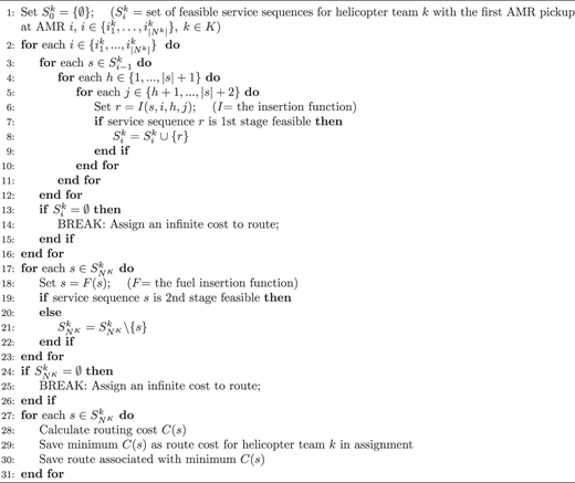
The AMR insertion algorithm with fuel insertion (see Algorithm 1) introduced in this paper addresses the rigid refueling feature by allowing for refuel stops at HLZs with refuel capabilities regardless if there is an associated AMR pickup or drop-off at the HLZ. The AMR insertion algorithm with fuel insertion introduces two separate feasibility checks. Similar to the AMR insertion algorithm, the first-stage feasibility occurs after each AMR insertion. Unlike the AMR insertion algorithm, this adapted algorithm does not verify aircraft fuel level feasibility in the first-stage feasibility check. Instead, the first-stage feasibility check includes AMR time windows, maximum passenger ride time, aircraft flight duration, aircraft capacity, and aircraft’s latest return to the airport feasibility. Only feasible routes are considered for the next AMR insertion. Upon insertion of all AMR pickups and drop-offs for the assigned AMRs to helicopter team k ∈ K, the algorithm produces a set of complete first-stage feasible routes , where Nk is the set of AMRs assigned to helicopter team k.
For each complete first-stage feasible route , the algorithm checks for aircraft team fuel feasibility. This is accomplished by ensuring that at every node j in complete route s, there is sufficient fuel to travel to node j + 1. If there is insufficient fuel to travel to the next node, the algorithm inserts a refueling stop between nodes j and j + 1. The algorithm selects the HLZ with refuel capabilities, not at node j or j + 1 which minimizes the travel time from node j to the refuel node plus the travel time from the refuel node to node j + 1 as the refuel stop. If there is not sufficient fuel at node j to travel to any HLZs with refueling capabilities, the complete route s is removed from .
The fuel insertion function generates a set of fuel-feasible complete routes, but the potential fuel insertions may have changed the time structure of the route. The fuel-feasible complete routes must go through a second-stage feasibility check to ensure the feasibility of AMR time windows, maximum passenger ride time, aircraft flight duration and aircraft’s latest return to the airport. Notice that the second-stage feasibility differs from the first in that the aircraft capacity need not be checked. The algorithm assumes no passengers board or deplane at the refuel insertions. Upon completion of the second-stage feasibility check, the algorithm either has a set of fully feasible complete routes to calculate routing costs or an empty set of fully feasible complete routes in which the algorithm assigns infinite cost to the route associated with the AMR assignment.
AMR insertion algorithm with fuel insertion
4.4 Feasible route limit and objective
Both the AMR insertion algorithm (Nelson et al., 2023a) and the AMR insertion algorithm with fuel insertion in Section 4.3 have the ability to create the optimal helicopter team routing for a given AMR assignment. This is due to the fact that both algorithms can generate and evaluate every possible AMR route sequencing. However, the number of routes to evaluate becomes intractable as the number of assigned AMRs increases. The largest instances encountered in practice correspond to approximately 100 AMRs (Nelson et al., 2023a). Including fuel insertion does not add to the time complexity of the original AMR insertion algorithm because it occurs outside of its main iterative loop. In order to solve larger problems, it is necessary to limit the number of feasible routes carried forward for the next AMR insertion.
The methodology in which we select τ feasible routes after each AMR insertion iteration to carry forward to the next iteration builds on the work done by Häme (2011) and is discussed in Nelson et al. (2023a). As the value of τ increases, so does the probability of generating a feasible route with a lower routing cost, but at an increased computational cost. We chose three candidate feasible route objectives to select the τ feasible routes to build upon at the next AMR insertion iteration. The first method chooses the τ routes with the smallest flight times. This is aligned with the third term of the problem’s overall objective (Nelson et al., 2023a, see Equation (1)) simplified here as,
and is shown in Equation (2). The other two feasible route objectives attempt to allow more flexibility in subsequent AMR insertions by choosing τ routes with either the maximum total slack time (3) or the maximum of the minimum slack times (4).
Given the routing sequence, r = (r1, …, rm), we wish to minimize the time of flight (TOF),
maximize the total slack time (TST),
or maximize the minimum slack time (MST),
where is the time between nodes j and j′ for helicopter team k, lj is the latest arrival time for the AMR j, and is the calculated time of arrival at node j.
4.5 Assignment improvement quantity ratio
The improvement cycle attempts to improve y assignments with the lowest overall objective values by attempting to shift unsupported AMRs to helicopter teams. An increase in y provides a greater opportunity to improve more initial assignments and therefore increase the potential to result in a better overall solution. A larger y also results in increased computation time and potentially less of the assignment space explored. We control the value of y by using parameter θ ∈ [0, 1] such that y = ⌊θζ⌋, where ζ is the initial AMR assignment quantity and .
5. Heuristic improvement design of experiments
5.1 Sequential experiments
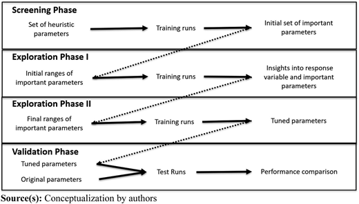
Gunawan et al. (2011) describe a sequential experimental approach to tune algorithm parameters. The approach includes screening, exploration, and exploitation phases to further tune parameters in order to improve algorithm performance. Figure 2 illustrates the air movement operations planning heuristic parameter tuning DOE procedure. The purpose of the DOEs is to analyze heuristic performance while varying the heuristic parameters in order to identify the best heuristic parameter settings. We design two scenarios with dissimilar HLZ networks and AMR demand to represent utility helicopter unit air movement operations. We tune the heuristic parameters (see Table 1) under each scenario and compare the resulting heuristic with tuned parameter settings performance. The interested reader can find the DOEs, phase results, and additional details in Nelson (2023) (see Ch. 3 and App C).
Parameters to tune
| Parameter | Data type |
|---|---|
| Initial AMR assignment quantity (ζ) | Discrete Numeric |
| Unrestricted assignment percent parameter (η) | Continuous |
| Aircraft team routing algorithm | Categorical |
| Feasible route limit (τ) | Discrete Numeric |
| Feasible route objective | Categorical |
| Assignment improvement ratio (θ) | Continuous |
The heuristic improvement DOE is a controlled set of tests designed to model and explore the relationship between the heuristic parameters and response variable (JMP and Proust, 2017; Montgomery, 2017). The primary response variable is the resulting overall objective value. Further analysis of the components of the overall objective value includes quantity and priority level of unsupported AMRs, aircraft team utilization penalty, and total flight time. The DOE sizes allow for 80% power for all main effects, second-degree interactions, and quadratic effects of all discrete numeric and continuous effects with 95% confidence for each phase.
5.1.1 Heuristic objective and penalty weights
The objective of the heuristic is to minimize the sum of weighted penalties of unsupported AMRs, helicopter team utilization and flight time. A heuristic objective formula that represents the mixed integer linear programming objective in Nelson et al. (2023a) is shown in Equation (5). The first summation in the objective accounts for the penalty of leaving AMRs unsupported. Let α be the unsupported penalty weight, bi be the transformed AMR priority for AMR i, and Πi be the binary variable with value 1 if AMR i is unsupported and 0 if supported. The second summation in the objective describes the penalties for helicopter team utilization and total flight time. Let βk represent the utilization penalty for helicopter team k and ϒk be the binary variable with value 1 if helicopter team k is assigned one or more AMRs and 0 if assigned zero AMRs to support. Let γk be the flight hour penalty for helicopter team k and Φk be the total flight hours for helicopter team k.
Similar to the practical application in Nelson et al. (2023a), the AMR priority level in this DOE is transformed through an exponential function with base B = 2. This implies that an AMR of one higher level priority is twice as important as an AMR of the priority level below. Let pi be the priority level of AMR i as referenced in Table A2. Then . We set the unsupported penalty weight α = 100, which can be interpreted as leaving an unsupported priority level 9 AMR as equivalent to logging 100 flight hours on a helicopter team with γk = 1. Setting α at a high value sets a priority of supporting all AMRs. The utilization penalty for each aircraft team βk is a calculated value used to balance the commander’s assessed cost of committing an aviation asset versus leaving an AMR unsupported. The calculation follows as . Given the commander’s AMR priority level threshold to launch a particular aircraft team for support, it is possible to calculate βk. This concept is discussed further in Section 6.2.2.
We define the expected AMR flight time for a given scenario as
where the HLZs are in the set , P(pickup = j) is the probability an AMR will originate at HLZ j, P(drop = j′|pickup = j) is the conditional probability the AMR drops off at HLZ j′ given the AMR picks up at HLZ j, and tjj′ is the flight time from HLZ j to HLZ j′.
6. Scenarios
6.1 Summary
We design two scenarios to tune the heuristic procedure with key differences in HLZ network scale and overall AMR volume. For each scenario, we define the HLZ network, refuel nodes, helicopter fleets, and AMR demand characteristics with identical distribution assumptions from Nelson et al. (2023a). The first scenario is a low-density operational environment set in Afghanistan whereas the second scenario features a small urban environment set in Baghdad, Iraq, serving a higher AMR volume. The expected AMR flight time of the Baghdad scenario is 0.1335 h, which differs significantly from that of the Afghanistan scenario’s expected AMR flight time of 0.51 h. Table 2 summarizes the major differences between the scenarios with the subsequent sections providing specific details.
6.2 Low-density scenario: regional command-north, Afghanistan
6.2.1 HLZ network
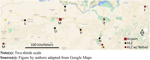
The HLZ network is a two-thirds scaled representation of Regional Command North, Afghanistan. The scaling is in order to allow the helicopter fleet to support a larger number of AMRs and thus further test the heuristic’s capabilities. As seen in Figure 3, there are ten HLZs, of which five have refueling capabilities. HLZs M and Z are hubs, serving as the pickup or drop-off HLZ for many AMRs.
(Color online) HLZ network for the scenario set in Regional Command North, Afghanistan
(Color online) HLZ network for the scenario set in Regional Command North, Afghanistan
6.2.2 Helicopter fleet
The helicopter fleet consists of six UH-60 Blackhawk helicopter teams stationed at HLZ M. Table 3 displays the helicopter team features. All teams have identical maximum passenger capacity, average cruising speed, and fuel capacity. There are two teams designated as AM with a flight window of 0700–1500. The two PM teams have a flight window of 1500–2100. Note that we assume the PM teams fly part of their mission under night vision goggles and therefore have a maximum duration of 6 h as opposed to the day-only AM team with a maximum duration of 8 h. The quick reaction force (QRF) teams straddle the AM and PM teams’ time windows with a flight window from 1100– 1900 and an 8 h maximum duration.
Regional Command – North scenario helicopter fleet
| Team | Earliest departure | Latest arrival | Max duration | Max capacity | Speed (km/hr) | Fuel (hours) | Utilization penalty (β) | Flight hour penalty (γ) |
|---|---|---|---|---|---|---|---|---|
| UH_AM_A | 0700 | 1500 | 8 | 22 | 222.2 | 2 | 1 | 1 |
| UH_AM_B | 0700 | 1500 | 8 | 22 | 222.2 | 2 | 1 | 1 |
| UH_PM_A | 1500 | 2100 | 6 | 22 | 222.2 | 2 | 1 | 1 |
| UH_PM_B | 1500 | 2100 | 6 | 22 | 222.2 | 2 | 1 | 1 |
| UH_QRF_A | 1100 | 1900 | 8 | 22 | 222.2 | 2 | 400 | 1 |
| UH_QRF_B | 1100 | 1900 | 8 | 22 | 222.2 | 2 | 400 | 1 |
The two helicopter teams designated with QRF can be considered high-cost teams. QRF helicopter teams are commonly used teams held in reserve, with crews that can rapidly react to any commander-directed missions. QRF teams are given air movement operation missions only when the commander deems the mission is of high enough priority to commit the reserve QRF asset. For this reason, the QRF helicopter teams are given a utilization penalty βk = 400, ∀k. This utilization penalty can be interpreted as the commander setting the QRF launch threshold equivalent to not supporting a level 7 priority (O-6 colonel or equivalent), two priority level 8 AMRs, or four priority level 9 AMRs since βk = 400 = (100)2(9–7) = (100)(2)2(9–8) = (100)(4)2(9–9), ∀k.
6.2.3 Air mission requests
For each run in the DOE, the number of AMRs is n = 30. The number of AMRs is set to stretch the limits of the low-cost helicopter teams in their ability to support the demand in a moderately large HLZ network. While each run has a fixed number of AMRs, the features of each run’s AMRs will differ. HLZs M and Z are hub HLZs serving as the pickup or drop off HLZ for many AMRs. The AMR feature distributions follow the practical application in Nelson et al. (2023a). Table A3 displays the Afghanistan scenario’s AMR HLZ pickup and drop-off probabilities.
The number of passengers per AMR is equally distributed between the integers from one to eleven. Each AMR has a 25% probability of having a priority level of 9, and a 25% probability of having a priority level of 8, with the remaining probability equally distributed among priority levels 1 to 7. Finally, each AMR is assigned a time window with equal probability for windows 0700–2100, 1200–1700, or 1700–2100. Finally, the maximum passenger ride time L is set at 4 h.
6.3 High-density scenario: Baghdad, Iraq
6.3.1 HLZ network
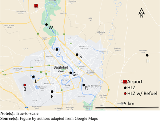
The Baghdad scenario HLZ network is a true-to-scale representation of the Multi-National Division – Baghdad, Iraq. As seen in Figure 4, the network consists of ten HLZs of which HLZs T and B have refueling capabilities. HLZs T, B, and L are hubs, serving as the pickup or drop-off HLZs for many AMRs.
6.3.2 Helicopter fleet
The helicopter fleet consists of six UH-60 Blackhawk helicopter teams stationed at HLZ T. The fleet is identical to the Afghanistan scenario fleet shown in Table 3 with speed as an exception. Due to the condensed nature of the HLZ network, helicopters travel slower on average in Baghdad than in a more spread-out HLZ network with speeds for all aircraft teams set to 185.2 (km/hr).
6.3.3 Air Mission Requests
For each run in the DOEs, the number of AMRs is n = 50. The number of AMRs is set to stretch the limits of the helicopter teams in their ability to support the demand even with high-cost QRF aircraft teams. HLZs T, B, and L are hub HLZs, serving as the pickup and drop-off HLZ for many AMRs. Due to the proximity of HLZs B and L and the fact they share a common forward operating base, there are no AMRs between the two HLZs. Table A4 depicts the AMR HLZ pickup and drop-off probabilities for the Baghdad scenario. The expected AMR flight time of the Baghdad scenario is 0.1335 h, which differs significantly from that of the Afghanistan scenario’s expected AMR flight time of 0.51 h.
The assignment of the number of passengers, priority level, and flight window for each AMR follows the Afghanistan scenario methodology as discussed in Section 6.2. Additionally, like the Afghanistan scenario, the maximum passenger ride time L is set at 4 h.
7. Heuristic improvement results
The heuristic improvement DOE sought to tune heuristic parameter settings in order to produce superior solutions to the Army aviation air movement mission assignment, utilization, and routing problem and improve on the heuristic presented by Nelson et al. (2023a). During the initial experiments for the Afghanistan scenario, a feasible route limit (τ) of 1 was not considered a good value and thus excluded in the initial screening range. Subsequent exploration phases showed τ = 1 to be the best value. With this in mind, the screening phase for the Baghdad scenario included this value in the initial DOE range for τ. The impact of this change removed any reason to do a second explore phase for the Baghdad scenario.
As shown Tables 4 and 5, the rigorous DOE process arrived at heuristic parameters tuned to two separate scenarios. The heuristic with tuned parameter settings resulted in solutions with lower objective values than those with its original settings. The tuned parameter settings in both scenarios provided statistically significant evidence of superior performance. Furthermore, the tuned parameter settings gained through separate scenario data sets, although slightly different, proved to produce similar solutions for both scenarios. Hence, using parameter settings tuned with Afghanistan scenario or Baghdad scenario training data is equally beneficial (see Table 6). The interested reader may consult Appendix B for details on solution quality over time.
Heuristic tuning results for the Afghanistan scenario
| Parameter | Screening phase | Explore I | Explore II | Validate |
|---|---|---|---|---|
| Initial AMR assignment quantity (ζ) | [500, 10,000] | [3,000, 7,000] | 7,000 | 7,000 |
| Unrestricted assignment percent parameter (η) | [50, 100] | 75 | 75 | 75 |
| Aircraft team routing algorithm | Constructive, Fuel Insertion | Fuel Insertion | Fuel Insertion | Fuel Insertion |
| Feasible route limit (τ) | [10, 500] | [5, 50] | [1, 5] | 1 |
| Feasible route objective | TOF, TST, MST | TST, MST | TST | TST |
| Assignment improvement ratio (θ) | [0.01, 0.1] | 0.01 | 0.01 | 0.01 |
| Scenario runs | 100 | 40 | 40 | 30 |
| Time per run (min) | 60 | 60 | 60 | 60 |
Note(s): Final tuned values are shown in the “Validate” column
Heuristic tuning results for the Baghdad scenario
| Parameter | Screening phase | Explore | Validate |
|---|---|---|---|
| Initial AMR assignment quantity (ζ) | [500, 10,000] | 10,000 | 10,000 |
| Unrestricted assignment percent parameter (η) | [50, 100] | 50 | 50 |
| Aircraft team routing algorithm | Constructive, Fuel Insertion | Constructive, Fuel Insertion | Fuel Insertion |
| Feasible route limit (τ) | [1, 500] | [1, 10] | 1 |
| Feasible route objective | TOF, TST, MST | TOF, TST, MST | TOF |
| Assignment improvement ratio (θ) | [0.01, 0.1] | 0.01 | 0.01 |
| Scenario runs | 100 | 40 | 30 |
| Time per run (min) | 60 | 60 | 60 |
Note(s): Final tuned values are shown in the “Validate” column
Original heuristic settings from Nelson et al. (2023a) and final tuned settings for each scenario
| Parameter | Original (Nelson et al., 2023a) | Afghanistan tuned | Baghdad tuned |
|---|---|---|---|
| Initial AMR assignment quantity (ζ) | 5,000 | 7,000 | 10,000 |
| Unrestricted assignment percent parameter (η) | 100 | 75 | 50 |
| Aircraft team routing algorithm | Constructive | Fuel Insertion | Fuel Insertion |
| Feasible route limit (τ) | 10 | 1 | 1 |
| Feasible route objective | TOF | TST | TOF |
| Assignment improvement ratio (θ) | 0.01 | 0.01 | 0.01 |
The motivated reader may find the instances for these DOEs and associated heuristic solutions in Nelson (2023, Appendix C, pp. 114–136).
To measure the improvement, we measure the objective value of the original heuristic from Nelson et al. (2023a) and the tuned validation settings for each of the 30 validation instances. Let D be the associated difference in objective values using Equation (5) and let μD be the true mean difference. The results of a paired t-test (Devore, 2016) for both scenarios strongly support that the objective value of the original settings is greater than the tuned settings (i.e. μD > 0). Table 7 provides the paired t-test results showing both sets of parameters result in improvement over the original parameters.
Paired t-test results comparing validation heuristic settings for each scenario to the original heuristic parameters from Nelson et al. (2023a)
| Improvement over original: Afghanistan scenario | Improvement over original: Baghdad scenario | ||
|---|---|---|---|
| D | p-value | D | p-value |
| 259 | 1.54 × 10⁻⁸ | 344.4 | 3.66 × 10⁻¹² |
For the Afghanistan scenario, 19 of 30 instances result in the tuned settings using one less high-cost QRF helicopter. The tuned parameters result in a lower objective value overall in 26 instances; in the four instances where this was not the case, the average difference was only 0.867 flight hours. On average the Baghdad-tuned settings supported all AMRs in all 30 instances where the original settings left 2.33 AMRs unsupported on average.
Numerical experiments with both tuned settings show similar performance both in terms of number of AMRs supported and total flight time. Using parameter settings tuned with either the Afghanistan or Baghdad scenario seems to be equally beneficial. The interested reader can review the numerical experiments in Nelson (2023, App C).
8. Application-sized problem
8.1 Overview
Nelson et al. (2023a) provide an application-sized problem as a proof of concept of the heuristic’s ability to generate feasible assignment and routing solutions in a time period useful to aviation mission planners. We now seek to generate comparable solutions in a condensed time period with tuned parameter settings on the identical scenario from Nelson et al. (2023a). The heuristic uses the Afghanistan scenario tuned parameter settings described in Table 4. Actual problem instances are available from Daniels et al. (2023).
8.2 Results
Table 8 provides the results and performance of the heuristic with original parameter settings – taken from Nelson et al. (2023a) – and the heuristic with Afghanistan scenario-tuned parameter settings (this paper) on identical application-sized problems. Both heuristics were able to find feasible solutions, supporting all AMRs for all instances in both 90 AMR and 100 AMR quantity-sized problems. The utilization and AMR support were identical for both heuristics. On average, the heuristic with tuned parameter settings arrived at assignment and routing solutions with 1.46 more hours of flight time, a 7.1% average increase. However, the heuristic with tuned parameter settings arrived at a solution in 22 min on average compared to the average 221-min execution time for the heuristic with original parameter settings. The drastically reduced execution time with minimal solution quality degradation provides aviation mission planners with opportunities to generate multiple courses of action (COAs) and perform additional mission analysis in a shortened mission planning cycle.
Application sized problem results with (left) heuristic from Nelson et al. (2023a) and (right) tuned settings from this paper
| n | Instance | Heuristic with original parameter settings from Nelson et al. (2023a) | Heuristic with Afghanistan scenario tuned parameter settings | ||||||||
|---|---|---|---|---|---|---|---|---|---|---|---|
| Time (s) | Objective | Unsupported | Utilization | Route time | Time (s) | Objective | Unsupported | Utilization | Route time | ||
| 90 | 1 | 13,326 | 30.80 | 0 | 10 | 20.80 | 1,616 | 31.34 | 0 | 10 | 21.34 |
| 90 | 2 | 10,364 | 29.87 | 0 | 10 | 19.87 | 954 | 32.09 | 0 | 10 | 22.09 |
| 90 | 3 | 5,086 | 31.15 | 0 | 10 | 21.15 | 689 | 30.62 | 0 | 10 | 20.62 |
| 90 | 4 | 12,134 | 29.10 | 0 | 10 | 19.10 | 1,681 | 31.29 | 0 | 10 | 21.29 |
| 90 | 5 | 10,085 | 30.51 | 0 | 10 | 20.51 | 1,048 | 30.99 | 0 | 10 | 20.99 |
| 90 | 6 | 3,654 | 31.73 | 0 | 10 | 21.73 | 405 | 34.60 | 0 | 10 | 24.60 |
| 90 | 7 | 11,996 | 30.48 | 0 | 10 | 20.48 | 1,288 | 31.36 | 0 | 10 | 21.36 |
| 90 | 8 | 7,375 | 29.77 | 0 | 10 | 19.77 | 801 | 32.84 | 0 | 10 | 22.84 |
| 90 | 9 | 11,304 | 29.36 | 0 | 10 | 19.36 | 1,239 | 30.36 | 0 | 10 | 20.36 |
| 90 | 10 | 8,280 | 28.88 | 0 | 10 | 18.88 | 800 | 31.00 | 0 | 10 | 21.00 |
| 100 | 1 | 14,755 | 31.59 | 0 | 10 | 21.59 | 1,180 | 33.06 | 0 | 10 | 23.06 |
| 100 | 2 | 19,265 | 30.81 | 0 | 10 | 20.81 | 2,404 | 32.26 | 0 | 10 | 22.26 |
| 100 | 3 | 15,124 | 30.57 | 0 | 10 | 20.57 | 1,461 | 31.78 | 0 | 10 | 21.78 |
| 100 | 4 | 19,538 | 29.11 | 0 | 10 | 19.11 | 2,145 | 31.42 | 0 | 10 | 21.42 |
| 100 | 5 | 19,929 | 33.83 | 0 | 10 | 23.83 | 1,107 | 35.23 | 0 | 10 | 25.23 |
| 100 | 6 | 20,680 | 30.23 | 0 | 10 | 20.23 | 2,416 | 31.06 | 0 | 10 | 21.06 |
| 100 | 7 | 20,360 | 32.17 | 0 | 10 | 22.17 | 943 | 33.64 | 0 | 10 | 23.64 |
| 100 | 8 | 8,531 | 32.52 | 0 | 10 | 22.52 | 803 | 34.38 | 0 | 10 | 24.38 |
| 100 | 9 | 15,634 | 31.28 | 0 | 10 | 21.28 | 786 | 32.62 | 0 | 10 | 22.62 |
| 100 | 10 | 17,654 | 29.49 | 0 | 10 | 19.49 | 2,214 | 30.54 | 0 | 10 | 20.54 |
Note(s): Problem instance data available from Daniels et al. (2023)
9. Conclusion
This paper sought to improve the air movement operations planning heuristic in order to generate superior solutions in less time. Through developing alternative modular methodologies and a rigorous DOE-based heuristic parameter tuning, we arrived at a fine-tuned heuristic with an average 33% objective improvement over the original heuristic described in Nelson et al. (2023a). The bulk of the objective improvement resulted from the reduced utilization of high-cost helicopter teams in the Afghanistan validation data set and through superior AMR support in the Baghdad validation data set. Improvements of this nature preserve costly and scarce army aviation, maintenance, and personnel assets while providing more services to supported units. Reduced high-cost aircraft team utilization frees the teams to conduct other command-directed missions and ultimately provides superior capabilities to the supported ground commanders. Additionally, during the Afghanistan scenario validation phase, the fine-tuned heuristic was able to provide a feasible solution in an average of 8.03 min, which is a 70% reduction in time compared to the original heuristic. Rapidly generated solutions enhance aviation mission planners’ ability to quickly generate COAs to meet the commander’s requirements. The dramatically reduced computation time also makes it feasible to employ distinct parameter sets for the objective function (e.g., α, B, βk, γk) to quickly generate multiple COAs for further analysis and/or refinement by the planners (Nelson et al., 2022).
9.1 Parameter tuning recommendations
In lieu of performing a full DOE approach to air movement operations planning heuristic parameter tuning, several general guidelines can be derived from experimentation. In operational scenarios where the number and type of AMRs exceed the support capabilities of the aircraft fleet, planners may encounter challenges in efficiently assigning and routing aircraft to support all AMRs or minimize the number of unsupported AMRs based on priority. The ability of the heuristic to generate feasible solutions would greatly aid in planning. To generate feasible solutions for such operational scenarios, users should configure the parameters to evaluate as many assignments as possible. Consequently, it is advisable to set the initial AMR assignment quantity (ζ) high, the unrestricted assignment percent parameter (η) to 100, the feasible route limit (τ) to 1, and minimize the assignment improvement quantity ratio (y).
Alternatively, if the aircraft fleet can accommodate numerous assignments with feasible routing, it may be advantageous to minimize helicopter team utilization and route time. This can be accomplished by reducing the unrestricted assignment percent parameter (η) and increasing the feasible route limit (τ) and assignment improvement quantity ratio (y).
9.2 Future work
There are many opportunities to further improve the air movement operations planning heuristic. It is reasonable to believe that the parallelization of the aircraft team routing process would significantly improve computational speed. Additionally, the heuristic should output useful products for the Army aviation mission planner and operator. To add additional sophistication, the heuristic could introduce flight characteristics associated with altitude and air temperature. Future efforts should consider approaches to adapt the heuristic parameters dynamically, or adjust the parameters based on scenario characteristics. Machine learning techniques may be worth exploring to improve heuristic sub-modules shown in Figure 1. Also, meta-heuristic techniques could be used to more effectively utilize improvements to instances found using the insertion algorithm. For example, evolutionary programming could combine the best portions of several instances to generate better solutions, while tabu search could more efficiently use the results of the insertion improvement algorithm. Future research should also consider designing a robust hyperparameter study focused on finding minimal regret hyperparameters for this heuristic across a broad range of operational scenarios (Eldar and Merhav, 2004; Yu and Zhu, 2020).
Finally, beyond solving the Army aviation air movement mission assignment, utilization, and routing problem, this heuristic has the potential to be integrated into additional decision support or planning models where estimating aviation demands or utilization is an important consideration. For example, the heuristic could assist in determining the best allocation of aviation resources to task forces (Nelson et al., 2023b). More generally, future efforts could apply similar types of refueling constraints to problems related to routing battery-powered vehicles that require regular recharging.
The first author was supported by an Omar N. Bradley Officer Research in Mathematics Fellowship. Additionally, Lieutenant Colonel Tyler Espinoza provided relevant and current insights into US Army aviation air movement operations. We also thank the anonymous reviewers for their comments and suggestions which led to improvements in the quality of the paper.
Disclaimer: Lieutenant Colonel Russell Nelson’s contribution was performed as part of his official duties as an employee of the US Government. The views expressed in this paper are those of the authors and do not reflect the official policy or position of the US Army, the Department of Defense or the US Government.
References
Appendix
A Additional informationA.1 Notation guide
Notation guide (in order of appearance within category)
| Sets | |
| K | set of helicopter teams |
| Nk | set of AMRs assigned to helicopter team k, |
| set of complete feasible routes for helicopter team k | |
| set of HLZs | |
| Indices | |
| i | index for AMRs, e.g., , in Algorithm 1 |
| indices for nodes in the HLZ network, j′ ≠ j | |
| k ∈ K | index for helicopter teams |
| s | index for route, |
| Parameters | |
| n | number of AMRs |
| βk | utilization penalty for aircraft team k, |
| initial AMR assignment quantity | |
| η ∈ [0, 100] | unrestricted assignment percent parameter |
| θ ∈ [0, 1] | assignment improvement quantity ratio |
| α | unsupported AMR penalty |
| γk | flight hour penalty for helicopter team k |
| B | base for exponential transformation of doctrinal AMR priority level |
| L | maximum ride time (hours) |
| Computational variables | |
| y | number of assignments to attempt to improve, y = ⌊θζ⌋ |
| τ | number of feasible routes after each AMR insertion iteration to carry forward to the next iteration |
| r = (r1, …, rm) | routing sequence |
| fTOF(r) | time of flight (TOF) for route sequence r |
| fTST(r) | total slack time (TST) for route sequence r |
| fMST(r) | minimum slack time (MST) for route sequence r |
| lj | latest arrival time for AMR j |
| time between nodes j and j′ for helicopter team k | |
| calculated time of arrival at node j | |
| bi | transformed AMR priority for AMR i, |
| Πi | binary variable with value 1 if AMR i is unsupported and 0 otherwise |
| ϒk | binary variable with value 1 if helicopter team k is assigned one or more AMRs and 0 otherwise |
| Φk | total flight hours for helicopter team k |
| pi | doctrinal AMR priority level from Table A2 |
Air mission request priority (pi) (Mogensen, 2014)
| AMR mission | Priority (pi) |
|---|---|
| Downed Aircraft Recovery | 1 (highest) |
| Emergency Leave | 2 |
| General Officer Movement | 3 |
| Military Working Dog | 4 |
| Critical Equipment Repair | 5 |
| Religious Services | 6 |
| O-6 Colonel or Equivalent | 7 |
| Rest & Recovery Leave | 8 |
| Other | 9 (lowest) |
A.2 Scenario Details
Additional scenario descriptions are available in Nelson (2023).
Afghanistan scenario AMR HLZ pickup and drop off probabilities
| HLZ | Probability pickup | Probability drop off given pickup HLZ | |||||||||
|---|---|---|---|---|---|---|---|---|---|---|---|
| M | A | S | U | G | Z | T | N | K | F | ||
| M | 1/4 | 0 | 1/9 | 1/9 | 1/9 | 1/9 | 1/9 | 1/9 | 1/9 | 1/9 | 1/9 |
| A | 1/16 | 1/4 | 0 | 1/14 | 1/14 | 1/14 | 1/4 | 1/14 | 1/14 | 1/14 | 1/14 |
| S | 1/16 | 1/4 | 1/14 | 0 | 1/14 | 1/14 | 1/4 | 1/14 | 1/14 | 1/14 | 1/14 |
| U | 1/16 | 1/4 | 1/14 | 1/14 | 0 | 1/14 | 1/4 | 1/14 | 1/14 | 1/14 | 1/14 |
| G | 1/16 | 1/4 | 1/14 | 1/14 | 1/14 | 0 | 1/4 | 1/14 | 1/14 | 1/14 | 1/14 |
| Z | 1/4 | 1/9 | 1/9 | 1/9 | 1/9 | 1/9 | 0 | 1/9 | 1/9 | 1/9 | 1/9 |
| T | 1/16 | 1/4 | 1/14 | 1/14 | 1/14 | 1/14 | 1/4 | 0 | 1/14 | 1/14 | 1/14 |
| N | 1/16 | 1/4 | 1/14 | 1/14 | 1/14 | 1/14 | 1/4 | 1/14 | 0 | 1/14 | 1/14 |
| K | 1/16 | 1/4 | 1/14 | 1/14 | 1/14 | 1/14 | 1/4 | 1/14 | 1/14 | 0 | 1/14 |
| F | 1/16 | 1/4 | 1/14 | 1/14 | 1/14 | 1/14 | 1/4 | 1/14 | 1/14 | 1/14 | 0 |
Baghdad scenario AMR HLZ pickup and drop off probabilities
| HLZ | Probability pickup | Probability drop off given pickup HLZ | |||||||||
|---|---|---|---|---|---|---|---|---|---|---|---|
| T | B | L | W | F | G | R | S | J | H | ||
| T | 1/6 | 0 | 1/4 | 1/4 | 1/14 | 1/14 | 1/14 | 1/14 | 1/14 | 1/14 | 1/14 |
| B | 1/6 | 1/3 | 0 | 0 | 2/21 | 2/21 | 2/21 | 2/21 | 2/21 | 2/21 | 2/21 |
| L | 1/6 | 1/3 | 0 | 0 | 2/21 | 2/21 | 2/21 | 2/21 | 2/21 | 2/21 | 2/21 |
| W | 1/14 | 1/6 | 1/6 | 1/6 | 0 | 1/12 | 1/12 | 1/12 | 1/12 | 1/12 | 1/12 |
| F | 1/14 | 1/6 | 1/6 | 1/6 | 1/12 | 0 | 1/12 | 1/12 | 1/12 | 1/12 | 1/12 |
| G | 1/14 | 1/6 | 1/6 | 1/6 | 1/12 | 1/12 | 0 | 1/12 | 1/12 | 1/12 | 1/12 |
| R | 1/14 | 1/6 | 1/6 | 1/6 | 1/12 | 1/12 | 1/12 | 0 | 1/12 | 1/12 | 1/12 |
| S | 1/14 | 1/6 | 1/6 | 1/6 | 1/12 | 1/12 | 1/12 | 1/12 | 0 | 1/12 | 1/12 |
| J | 1/14 | 1/6 | 1/6 | 1/6 | 1/12 | 1/12 | 1/12 | 1/12 | 1/12 | 0 | 1/12 |
| H | 1/14 | 1/6 | 1/6 | 1/6 | 1/12 | 1/12 | 1/12 | 1/12 | 1/12 | 1/12 | 0 |
B Solution quality over time
B.1 Overview
During heuristic improvement through parameter tuning design of experiments, we fixed each run at 60 min. Throughout the run time, the heuristic had the ability to update the solution and improve the overall objective. We chose the 60-min run time as a time frame that would be acceptable for an aviation air mission operations planner during typical operational conditions. We also analyze how the quality of the solution improves over a longer period of time. This will give further insight into how the mission planner could choose to use the air movement operations planning heuristic based on mission and planning conditions.
In this analysis, we use the heuristic with Afghanistan scenario tuned heuristic parameter settings as described in Table 6. We allow the heuristic to run for six hours on each of the thirty Afghanistan Scenario validation data runs described in Section 6.2.
B.2 Results
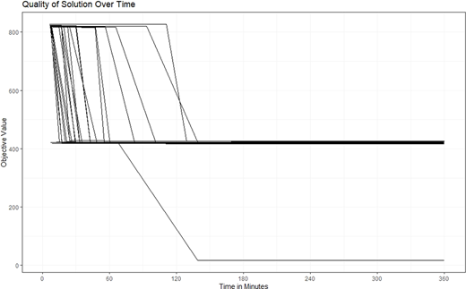
Figure A1 displays the results of the quality of solution over time analysis. The lines show the best objective values for each of the 30 runs over the six-hour execution time. An objective value decrease of 400 or more represents a solution that uses one less high-cost QRF helicopter team. Smaller objective value decreases are gained through route time improvements. The graph shows five runs that had significant objective value improvements (a decrease of at least 400) after the 60-min mark. This leaves the heuristic obtaining the best solution for twenty-five of the thirty runs within the first hour. Furthermore, the heuristic obtained its best solution for all runs within 150 min. Following the results of this analysis, the aviation mission planner should have confidence that a 60-min run time will have greater than 83% probability (confidence interval [65.3%, 94.4%]) of finding the best heuristic solution and even greater probability (confidence interval [88.4%, 100%]) with a 150 min run time.