CAPM verification using overnight and daytime returns

The capital asset pricing model (CAPM) indicates a linear relationship between the expected return and systematic risk(referred to as the stock market beta). Numerous empirical analyzes have been conducted on this topic. Black et al. (1972) used the portfolio beta for cross-sectional analysis to establish the validity of the CAPM model. They revealed that the security market line of the US stock market has a flatter slope than that predicted by CAPM. Fama and MacBeth (1973) used the monthly return of stocks traded in the US stock market and validated a linear relationship between the expected return and systematic risk. Their conclusion regarding the slope does not differ from that of Black et al. (1972).

Recent studies have focused on the appearance of a positive relationship between the return and beta. Cohen et al. (2005) indicated a positive relationship between the return and beta during high inflation and a negative relation during low inflation. Savor and Wilson (2014) argued that a statistically and economically significant positive relation exists between the return and beta when announcements regarding inflation, unemployment rates, or Federal Open Market Committee’s benchmark interest rate decisions are scheduled. Jylla (2018) demonstrated a positive slope of the security market line when investors’ borrowing conditions are moderate and a negative slope when investors’ borrowing conditions are strict.

These results are identical to Black’s (1972, 1992) claim that if the CAPM’s assumption of investors being able to borrow money at a risk-free rate is not satisfied, the slope of the security market line will be flatter than expected. Black explained that investors with leverage constraints build their portfolio with higher betas, and hence, stocks with high betas require a relatively low-risk premium.

Hendershott et al. (2019) examined the relationship between the returns and beta on the daily data. They determined that the security market line is negative when using the daytime return, i.e. returns from open price to close price of a day, whereas the security market line is positive when using overnight return, i.e. returns from the close price of the previous day to the open price of the preceding day. Such phenomena are not limited to the US stock market but to other stock markets such as that of the EU.

Hendershott et al. (2019) described this phenomenon as a result of speculative behaviors of day traders. These day traders with speculative tendencies short sell low-beta stocks and buy high-beta stocks when the market opens and clears their portfolios before the market closes in the afternoon due to leverage constraints. Therefore, during the daytime when stocks are being traded, high-beta stocks require relatively lower risk premiums; at night when stocks are not traded, higher systematic risk (i.e. stocks with higher beta values)is required for relatively high-risk premiums. Therefore, the slope of the security market lines calculated using the daytime returns and that using the overnight returns differ.

In the Korean stock market, most major global stocks are traded during the night when most Korean investors are unable to trade, and the effect of this is indicated in Table 1. KOSPI_CO is the log return of the KOSPI index’s closing price for the day’s closing price compared with the previous day’s close, and KOSPI_OC is the log return of the KOSPI index’s closing price of the day compared with the opening price of the same day. A correlation of 0.733 exists between S&P 500 and KOSPI_CO, and the correlation between the S&P 500 and KOSPI_OC is negative, suggesting that the influence of the global stock market is mostly reflected in the domestic stock market. Therefore, as the influence of the global stock market is mostly reflected in the Korean stock market, which has a relatively high dependency on the global market, beta is reflected in the log return of the KOSPI index’s closing price of the day compared with the opening price of the same day more during the night than during the daytime. Considering such a phenomenon, it can be inferred that the slopes of the security market line for daytime returns and overnight returns differ in the Korean stock market.

Looking at the variance-covariance from Table 1, the proportion of the daily KOSPI returns on the current day’s opening price compared with the previous day’s closing price is (2.052%–0.140%)/4.701%, which is 40.7%. This implies that the overnight return significantly impacts the volatility of the Korean stock market, suggesting that decomposing daily returns into daytime and overnight returns would be meaningful.

Based on the research conducted by Hendershott et al. (2019), this study derives stock market security lines from the overnight and daytime returns in the Korean stock market and confirms the slope difference between the two. In addition, the suitability of beta is reviewed by comparing different beta calculation methods. The comparison of the outcomes of the two strategies in the Korean market is examined: a trading strategy based on the results of this study and the low beta/low-volatility trading strategy, which is a representative smart beta strategy. The rest of this paper is organized as follows. Section 2 introduces a method for deriving the security market line using individual stock return data. Section 3 derives the security market line and investigates whether the beta differently affects daytime and overnight returns. Finally, Section 4 summarizes the results of this study and suggests implications and further research directions.

In the study, decile portfolios are constructed in accordance with daily, overnight and daytime betas of individual stocks. By obtaining the average beta of the portfolios and monthly futures daily, overnight and daytime returns, three security market lines, respectively, are derived. The daytime beta is computed by the individual stock’s return between the opening price and the closing price of the same day, along with the return between the KOSPI index’s opening price and the closing price of the same day. The overnight beta is computed from the individual stock’s return between the previous day’s closing price and the next day’s opening price return in combination with the return between the previous day’s closing price of the KOSPI index and the current day’s closing price of the KOSPI index. Finally, the daily beta is derived from the individual stock’s return between the closing price of the previous day and the closing price of the next day, as well as the return between the KOSPI index’s closing price of the previous day and the closing price of the next day.

The data used in the study are as follows. The data sample is from late December 2000 to the last day of October 2019 for the stocks selected on the last trading day of each month. The selected stocks are those listed in the Korean Stock Exchange (KRX) with (1) a market capitalization greater than 50bn won, (2) a 20-day average trading volume of more than 500m won and (3) listed on the stock market for more than one full year. Stocks under a trading haul of any kind are excluded. Minimum market capitalization and transaction volume conditions are set to ensure that any sizable investments on these stocks are meaningfully reflected in the data. Furthermore, one full year listing restrictions are applied for the accumulation of sufficient data points for beta estimation. The essential market data such as adjusted stock prices, financials and accounting data are extracted from the data guide.

For beta calculations of the individual stocks (i), the daily/daytime/overnight returns of the individual stocks are as follows:

As a proxy for the market portfolio for beta calculation of individual stocks, the KOSPI index, which represents the performance of all stocks listed on the securities market is used and the return calculations are as follows.

The daily beta value $βi,tC$of an individual stock (i) is calculated based on the slope computed through regression analysis using the past year’s $Ri,tC$ and $Rm,tC$⁠. The daytime beta value $βi,tD$ is calculated based on the slope computed through regression analysis using the past year’s $Ri,tD$ and $Rm,tD$⁠. The overnight return $βi,tN$ is obtained based on the slope computed through regression analysis using the past year’s$Ri,tN$ and $Ri,tN$⁠. Although beta in CAPM is calculated with risk premiums, risk-free return is not considered in this analysis because the daily risk-free return is of negligible value. In fact, no difference exists in betas regardless of whether the daily risk-free return is subtracted. Hendershott et al. (2019) calculated beta values without deducting daily risk-free rates. Based on the three beta values, the stocks subject to analysis are divided into decile portfolios, i.e.10 portfolios. Portfolio betas are obtained by averaging betas of the individual stocks included in each portfolio. Equation (1) calculates the return of each individual stock (i) by accumulating the monthly return, the monthly daytime return and the monthly overnight return from the last trading day of each month to the last trading day of the following month. Furthermore, the equation calculates the average returns of each individual stock in the portfolio, which is used as the portfolio’s monthly/daytime/overnight returns in the following month.

For the 10 portfolios created on the basis of the daily beta, the relation between the portfolio daily beta and the portfolio’s daily, daytime and overnight returns in the next month is analyzed and the same is done for the portfolio’s daytime beta and overnight beta. A panel regression analysis as in equation (3) is performed to analyze the difference between the slopes of the security market line calculated from the daytime and overnight returns.

If D_t+1 is the daytime return, it is a dummy variable that equals 1 and f_t+1 is the fixed effect on the date. $β^i,tp$ is the portfolio beta.

Market capitalization at the base date is used as an indicator to identify the characteristics of individual stocks. B/P is calculated by dividing the most recently announced quarterly net assets by the base date’s market capitalization. Considering the time lag of the quarterly performance announcement, the quarterly asset value data is taken from at least two months earlier. Momentum is calculated using the adjusted stock price by subtracting the latest month’s return from the past year’s return. Volatility is taken from Dataguide, which uses the weekly return in the past year. The statistics of each portfolio is as seen in Table 2.

Portfolios with high beta, as seen in Table 2, appear to have high volatility and low momentum. This implies that while beta represents relative volatility to the benchmark, the large beta group indicates high volatility due to absolutely low momentum. The stocks with a higher beta are relatively larger in size; however, stocks with a smaller market cap receive relatively low attention from traders and trading volumes. Therefore, the benchmarking movement slightly impacts the changes in these individual stocks. Considering that there exists significant analyst coverage and a large number of investors for stocks with a larger market capitalization, it implies that the benchmarking movement and other information are reflected rather quickly. Thus, the beta value that indicates sensitivity to the benchmark is also large. While B/P value difference is usually not significant depending on the size of the beta, the group with a relatively average beta also has a high B/P value.

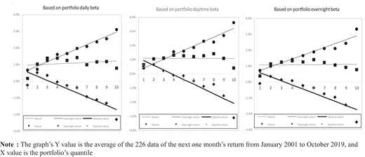
To verify the CAPM by splitting into the daytime and overnight returns, the next month’s monthly/daytime/overnight return is calculated for the portfolio divided into daily/daytime/overnight beta. The results are indicated in Table 3 and Figure 1.

As indicated in Table 3, portfolios with high beta have better overnight returns and lower daytime returns. The results are the same across all the portfolios based on daily/daytime/overnight betas. While beta does not affect returns as much, the portfolio with the highest beta and that with the lowest beta indicates relatively lower one-month returns. As indicated in Table 2, the portfolio with the lowest beta indicates a relatively high momentum but also a mean-reversion phenomenon in the short-term return. The portfolio with the highest beta, which usually has relatively high volatility, displays low returns due to the low volatility anomaly.

As indicated in Figure 1, the slope of the security market line calculated using the overnight return is positive and the slope calculated using the daytime return is negative. This does not make any difference even when the beta calculation method changes. Furthermore, the slope of the security market line close to 0 indicates that systematic risk also referred to as beta, minimally impacts returns. As the slope of the security market line calculated using the overnight return is positive, the systematic risk seems to be mostly reflected in the day’s opening price compared with the previous day’s closing price. The returns from the opening to the closing on the same day show a reverting behavior due to the overshooting at the opening price. This reverting pattern can be explained by the speculative day traders’ portfolio clearing at the closing price. Furthermore, after the systematic risk is reflected in the opening price, the price of individual stocks during the trading day is driven by the news for individual stocks. Therefore high-beta portfolio underperforms due to low volatility anomalies.

Although the security market line in Figure 1 only has 10 data points, to validate the security market line, a regression analysis is conducted as in Formula 4. In calculating the next month’s return, both equal-weighted return and value-weighted returns are applied. The result of the analysis performed for each of them is shown in Table 4.

Both the negative slope of the security market line calculated using daytime returns and the positive slope calculated using overnight returns are statistically significant. In particular, the t-statistic and R-squared values of the slope of the security market line computed using overnight returns are relatively high. This result implies that most factors that influence the fluctuation in returns can be explained by the systematic risk (reaction to changes in the global market), which is the return from the previous day’s closing price compared with the current day’s opening price. This indicates that beta has strong explanatory power. Hence, CAPM can be a useful model in explaining the overnight returns of the stocks listed in the Korean stock market. Furthermore, the effect of systematic risk in the daytime and overnight returns on individual stocks is observed to be different. The same results are obtained when the return of the portfolio is calculated using the value-weighted method of the individual stocks. Finally, the slope of the security market line computed based on returns is the sum of the two slopes calculated using overnight returns and daytime returns. It shows no statistical significance, which is not very different from the result of previous studies. When analyzing different beta calculation methods, beta calculation using overnight return indicates relatively high t-statistics and R-squared values. This implies that it is much more useful to calculate the beta of individual stocks based on the return of the current day’s opening price to the previous day’s closing price, which is mainly affected by systematic risk.

For a more detailed analysis, a Fama–MacBeth regression analysis as in equation (5) is performed. An analysis of daytime and overnight returns is performed to confirm the difference in the slopes. Using the overnight beta, the individual stocks are split into 10 decile portfolios and to calculate Equation (5)’s portfolio beta, a regression analysis of the monthly returns of the past 60 months is performed. The results are indicated in Table 5.

The slope of the security market line computed from the daytime return in Table 5 is −3.7%, implying that for every increase in beta by 1, the monthly average daytime return decreases by 3.7% with statistical significance. The slope of the security market line using overnight return, in the case of equal-weighted criteria, is 3.2%. The results are no different on a value-weighted basis.

Regression analysis as in equation (3) is performed to analyze the slopes of the security market line using daytime and overnight returns. A dummy variable with a daytime return of 1 is added to the explanatory variable to control the difference in the daytime and overnight returns. The results are indicated in Table 6. The slope difference is a factor of Day × β and depending on the beta calculation method, it is between 0.037 and −0.054 and is statistically significant. Similar to the regression analysis, a panel analysis indicates a statistically significant result in the beta on overnight returns.

Combining the results of the regression, Fama–MacBeth regression and panel analyzes, CAPM indicates a positive slope of the security market line computed using overnight returns in the Korean stock market. The slope of the security market line computed from daytime returns is negative. Finally, the systematic risk or beta, computed from overnight returns better explains the relation between individual stocks and market returns.

In addition to 10 portfolios on beta, an analysis of 25 portfolios based on market capitalization and B/P is performed. The industry classification of individual stocks is conducted based on 10 industries in FICS provided by FnGuide. Adopting the method used by Fama and French (1992), 25 portfolios are constructed based on market capitalization and B/P. B/P is calculated by dividing the quarterly total capital by market capitalization, where the total capital value in the prior two months at least is used due to the publication lag. A regression analysis and Fama–MacBeth regression analysis is conducted in a similar fashion as in the previous section, and the results are indicated in Table 7.

Even after considering the industries, market capitalization and B/P, beta value and daytime return indicate a negative relation, while beta value and overnight return show a positive relationship; this is statistically significant. In the case of the equal-weighted return, the difference between the two slopes of the security market line calculated using daytime and overnight returns is 0.043, which is almost the same as the slope difference in the Fama–MacBeth regression analysis. Furthermore, the difference between the two slopes is statistically significant, and the analysis based on the value-weighted returns yields the same results.

Then, an analysis is performed to examine the difference in the daytime and overnight returns after controlling for the effect of major factors of the individual stocks such as market capitalization, B/P, momentum and volatility. The target groups are divided into quintiles based on the four factors mentioned previously, and each quintile is also again divided based on betas. An observation is made to observe any differences between the low beta quintile’s daytime return and high beta quintile’s daytime return, and observation is also made to see if there are differences between the low beta quintile’s overnight return and high beta quintile’s overnight return. Here, the beta is computed from the overnight return. The return of the 25 quartiles of the portfolio’s return is based on the equal-weighted returns of the individual stocks, and the results are indicated in Table 8.

When the low-beta and high-beta portfolios are divided into quintiles based on market capitalization, the daytime return is better in the low-beta portfolios with the exception of the low market cap stocks. Further, the difference between the portfolio with the lowest beta and that with the highest beta is statistically significant. The low-beta portfolios have better daytime return even when they are compared based on B/P, momentum and volatility quintiles and the higher-beta portfolios indicate better overnight returns, which are statistically significant. However, for the stocks in the top quintile of volatility, a larger difference exists in returns compared with the other segments and in particular, the relation between beta and return is different.

Based on the fact that beta differently impacts the daytime and overnight returns, the performance of the zero-cost trading strategy is analyzed. Once the stock market opens, of the 10 portfolios sorted by beta size, the portfolio with the smallest beta is bought and the portfolio with the largest beta is shorted. When the stock market closes, the opposite condition is considered. In other words, the portfolio with the highest beta is bought and the portfolio with the lowest beta is shorted. Table 9 presents descriptive statistics on the performance of the strategy. By the beta calculation method, the daytime return is between 2.24% and 3.77%; the overnight return is between 2.32% and 3.04% and the return is between 4.61% and 6.96%. The results are similar even when value-weighted return is applied. Of the zero-cost portfolio returns, the trading strategy using beta computed using overnight returns indicates the best performance.

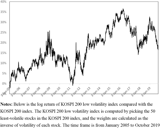
Next, the zero-cost trading strategy and low-beta strategy are compared. The low-beta strategy is conducted by buying the portfolio with the lowest beta value at the end of every month and shorting the portfolio with the highest beta of the 10 portfolios sorted by beta value and holding it for the next whole month. The low-beta method, as in Table 10 indicates consistent results until 2015 but fails to continue to produce stable results after 2016. Considering that most low volatility stocks are also low beta, the results are similar to Figure 2 which is the return of the low volatility index. Figure 2 depicts the trend of the excess performance of the K200 low volatility index against the K200 index released by the Korean stock exchange. While the smart beta strategy, a representative of the low volatility/beta strategy, has failed to yield positive results, the strategy of buying a low-beta portfolio during the daytime and buying the high-beta portfolio overnight has shown to consistently produce positive results. This implies that beta still affects the daytime and overnight returns in different ways.

Hendershott et al. (2019) revealed that the US and international stock markets have a different correlation between individual stocks and the beta in the daytime and overnight, and this is confirmed in the Korean stock market. The overnight return, the return between the previous day’s closing price and the opening price of the preceding day, indicates a positive relation between beta and the return. Furthermore, the daily return, the sum of the daytime and overnight returns, indicates no significant relation with beta. This proves that CAPM is useful for explaining the overnight return when the market is closed. We indicated that the result is the same after controlling for common factors such as industry classification, Fama–French classifications and so on.

For beta calculation, three methods are used: the return from the previous day’s closing price to the preceding day’s closing price; the return from the previous day’s closing price to the current day’s opening price; and the return from the opening price to the same day’s closing price. All three betas indicate a positive relationship with the overnight return, a negative relation with the daytime return and no significant relation with the overall return. In particular, when using the previous day’s closing price and the current opening price to calculate the beta, the analysis presents a more statistically significant result and a higher R-squared value. Overnight returns are mostly affected by common factors or systematic risks such as global stock rather than stock-specific risks. Therefore, the effect of return on systematic risk explained by CAPM is found to be more useful for beta calculated from data intervals, with a high impact on systematic risk. This is an additional achievement in that the analysis has been applied to the Korean stock market using Hendershott et al.’s (2019) analysis method. The zero-cost trading strategy based on the findings works in the same way. This paper’s additional contribution is the comparative analysis using the smart beta strategy. Through the comparison with the zero-cost trading strategy, it is confirmed that the effects of betas on daytime and overnight returns are still different. The typical smart beta strategy of low volatility and low beta fails to work after 2016 in the Korean stock market.

We find that 40% of daily returns are from overnight returns and that the daytime and overnight returns behave in different ways. Therefore, it is practically meaningful to split daily returns into daytime and overnight returns in many asset pricing applications. For example, the study by Shim (2018), which investigates higher moment risks such as skewness and stock return, can be extended to the higher moment risk measures on daytime or overnight returns.