Mean–variance relationship and uncertainty

Many studies have shown interest in models with rational investors in financial markets and have developed models to explain anomalies in financial markets. Based on classical finance theories, taking a high risk is compensated with high returns, consistent with a positive mean–variance relationship. However, the ambiguous mean–variance relationship has been argued for decades (French et al., 1987; Campbell, 1987; Turner et al., 1989). Additionally, some literature argues the effect of behavioral biases of investors on the mean–variance relationship (Cohen et al., 2005; Yu and Yuan, 2011; Kim et al., 2017a; Seo et al., 2021) to explain this unclear relationship.

The theory of rational asset pricing insists on a positive mean–variance relationship. Merton (1973) shows a positive relationship between the conditional expected excess stock returns and the conditional variance in the intertemporal capital asset pricing model. The literature, including French et al. (1987), Bailie and De Gennaro (1990), Ghysel et al. (2005) and Pástor et al. (2008), finds empirical evidence supporting this positive mean–variance relationship. However, some studies, including Campbell (1987), Nelson (1991) and Brandt and Kang (2004), discover a negative mean–variance relationship. Turner et al. (1989) and Glosten et al. (1993) provide empirical evidence of both a positive and negative relationship.

Uncertainty is an important concept in finance, accompanied by much literature on its impact on asset price movements. Buraschi and Jiltsov (2006) show that the model uncertainty induced by heterogeneous agents explains better dynamics of option prices and volume than the models with stochastic volatility. Andersen et al. (2009) find empirical evidence that uncertainty seems to be different from risk and seems to have a different impact on asset prices, compared with risk. Some literature suggests the measure of uncertainty. Baker et al. (2016) develop economic policy uncertainty (EPU) ^[1] based on news. They show that EPU contains information on the movements in policy-related economic uncertainty. Based on EPU, many studies including Pástor and Veronesi (2013), Brogaard and Detzel (2015) and Arouri et al. (2016) confirm that EPU exerts influence on risk premium. In addition, Baltussen et al. (2018) propose the measurement of uncertainty about risk, the volatility-of-volatility (VOV) ^[2], and show that the stocks with low VOV outperform the stocks with high VOV. Based on VOV, Hollstein et al. (2019) show that time-varying VOV commands a significant negative risk premium after controlling for volatility and jump risk. Ruan (2020) provides empirical evidence that there is a significant negative relationship between equity option returns and VOV after controlling for numerous option and stock characteristics. In this study, we focus on the influence of uncertainty on the risk–return relationship in the stock market.

Since uncertainty plays an important role in asset pricing, some literature explores the effect of uncertainty on the mean–variance relationship. Yang and Yang (2021) show the impact of EPU on the mean–variance relationship in the Chinese stock market. They find that the stock market's excess return is positively (negatively) related to conditional variance during low (high) EPU periods. However, they use only one uncertainty measure to provide direct evidence of the mean–variance relationship with conditional variances. Moreover, they do not consider the influence of other factors on the mean–variance relationship, as investigated in previous literature.

This study employs not only EPU but also the VOV to measure uncertainty in the stock market. We utilize the model-free implied variance from the options market as future stock market return variance in addition to four conditional variances estimated based on historical stock market returns. We also check the return–innovation relationship to provide additional indirect empirical evidence of the mean–variance relationship and consider the information of investor sentiment ^[3] to identify unique information of uncertainty on the mean–variance relationship.

Along with Yang and Yang (2021), we expect high EPU to distort the positive mean–variance relationship. EPU increases investors' uncertainty aversions and risk perceptions and changes in the firm's fundamental information ^[4]. While both EPU and VOV generally contain information on uncertainty, VOV reveals uncertainty about risk, which is different from the government's policy uncertainty in EPU. Therefore, the mechanism by which VOV affects the stock market's mean–variance relationship is different from that of the EPU.

In addition, we also conjecture that high VOV weakens the positive mean–variance relationship. Park (2015) shows that the negative skewness in the return distribution is proportional to the VOV, and the excess kurtosis in the return distribution is proportional to the squared VOV. Thus, he proposes VOV as a tail risk indicator in his model and argues that an increase in VOV would raise the prices of tail risk hedging options and lower subsequent returns. The extent of uncertainty about risk is a critical factor for determining the likelihood of meager returns. Through the stochastic channel (i.e. a persistent volatility process with a leverage effect), VOV can reveal the degree of the market's perception of tail risk incorporated into stock market dynamics. As an increase in VOV associated with the leverage effect of Black (1976) and Christie (1982) causes a negative mean–variance relationship ^[5], a positive risk–return tradeoff is undermined during the period of high VOV.

Collectively, we hypothesize that a positive relationship between the expected stock market return and variance is invalidated in periods of high uncertainty (i.e. periods of high EPU or high VOV). Still, this relationship is restored in low uncertainty periods (i.e. periods of low EPU or low VOV). Following Yu and Yuan (2011), we analyze the mean–variance relationship within high and low uncertainty regimes to test the hypotheses. In high uncertainty periods, we find the mean–variance tradeoff to be significantly negative. In contrast, during low uncertainty periods, a positive risk–return tradeoff is observed. Further evidence that the effect of uncertainty is critical for the risk–return tradeoff occurs in the reactions of stock market returns to variance innovations. During periods of high uncertainty, a negative relationship between returns and contemporaneous innovations of conditional variances and a positive relationship between returns and contemporaneous innovations of implied variance are significantly weakened. These results are consistent with changes in investors' uncertainty aversion, investors' risk perceptions, the firm's cash flow risk, investment risk and the leverage effect generated by the uncertainty shock. In low uncertainty periods, the return is negatively related to contemporaneous innovations of conditional variances and positively related to contemporaneous innovations of implied variance, consistent with the positive mean–variance relationship we show during such periods. The results are robust to changing the base assets to construct a mimicking factor for uncertainty and removing the effect of investor sentiment on the mimicking factor for uncertainty.

This study contributes to the literature on uncertainty by proving that uncertainty plays an important role in empirical asset pricing. First, we extend the uncertainty measures beyond EPU. EPU is a news-based measure constructed based on text mining techniques; it lacks investors' perspectives in the stock market. However, VOV offers various advantages over uncertainty measure based on articles in newspapers: it is ex ante, easy to compute, extracted directly from the options market, includes information on future underlying asset movements, available at a daily frequency and circumvents the self-selection problem in articles in newspapers (Just and Crigler, 1989). Additionally, our study suggests a novel mechanism for uncertainty derived from the options market to movements in the stock market. Second, we employ the model-free implied variance extracted from options prices in addition to the conditional variances estimated based on historical stock market returns. Many studies document that implied volatility contains superior information that can help forecast future volatility (Christensen and Prabhala, 1998; Blair et al., 2001; Jiang and Tian, 2005; Busch et al., 2011). Therefore, exploiting the implied variance can help confirm the information of uncertainty on the stock market movements more strongly. Third, we provide additional indirect evidence based on the return–innovation relationship analysis to confirm the impact of uncertainty on a positive risk–return tradeoff. Lastly, as Yu and Yuan (2011) show high sentiment undermines a positive mean–variance tradeoff; we check whether uncertainty has unique and additional information on the risk–return tradeoff beyond investor sentiment.

The remainder of this paper is organized as follows. Section 2 introduces the uncertainty measures and the methodology used to create the mimicking factor for the uncertainty measures. Section 3 describes the data and presents the main empirical results. Section 4 discusses the robustness checks. Finally, Section 5 concludes the paper.

This section introduces the uncertainty measures and the methodology used to form a mimicking factor to track uncertainty. We also introduce the conditional variances and implied variance mainly investigated in this study.

Baker et al. (2016) develop an EPU to gauge policy uncertainty shocks. They construct the United States (US) EPU based on search results from articles of 10 prominent newspapers: USA Today, Miami Herald, Chicago Tribune, The Washington Post, Los Angeles Times, The Boston Globe, San Francisco Chronicle, The Dallas Morning News, Houston Chronicle and The Wall Street Journal. Notably, the US EPU is calculated based on normalizing the number of articles containing at least one term related to economic and policy uncertainty such as “uncertainty” or “uncertain,” “economic” or “economy,” and one or more among the following terms: “congress,” “legislation,” “white house,” “regulation,” “federal reserve” or “deficit.”

Baltussen et al. (2018) propose VOV to measure uncertainty about risk. They argue that as VOV gauges dispersed investors' subjective beliefs about the volatility of expected stock return distribution, it could capture the uncertainty about the risk perceived by investors. Specifically, the implied volatility extracted from options prices is regarded as the expected stock return volatility, and VOV is computed as the standard deviation of implied volatility scaled by average implied volatility. Therefore, we employ the VOV on day t, calculated as follows:

where $σt¯IV=120∑i=t−19tσi,$ and $σi$ is the implied volatility on day i.

Following empirical asset pricing literature, including Ang et al. (2006) and Kapadia (2011), we construct a mimicking factor to measure the exposure to uncertainty by estimating the coefficient b^’ in the following regression:

where EPU_t (VOV_t) is the EPU (VOV) in month t, and X_t is the set of returns on the base assets in month t. Following Kapadia (2011), we use the Fama–French three factors as base assets. Based on the estimation of equation (2), the mimicking factor for EPU (FEPU) or VOV (FVOV) in month t is defined as:

where $bˆ′$ is the coefficient estimate of b^′. Based on FEPU and FVOV, we analyze the effect of uncertainty on the mean–variance relationship.

French et al. (1987) find empirical evidence of a positive relationship between the expected market risk premium and the volatility estimated by the rolling window model. Following them, we employ the realized variance based on the daily returns in month t as the conditional variance of the return on the next month t+1:

where Var_t(R_t+1) is the estimate of the stock market return variance for the next month t+1 based on conditional information at month t. e(t) is the last day of the month t, r_e(t)−d is the demeaned return on the day (e(t)−d), with subtraction of the average daily return during month t and N_t is the number of trading days in month t.

Ghysel et al. (2005) introduce the mixed data sampling (MIDAS) model to estimate monthly conditional variance forecasts with past daily returns. Following them, we employ the conditional variance estimator of the MIDAS with the exponential Almon lag specifications (Almon, 1965; Judge et al., 1985) as follows:

where $wd(κ1,κ2)=exp(κ1d+κ2d2)∑i=1252exp(κ1i+κ2i2),$e(t) is the last day of the month t, and r_e(t)+1−d is the return on the day (e(t)+1−d). We obtain the monthly conditional variance forecast using the daily data of the previous 252 days with the parameter estimates from the rolling window estimation with the previous 252 daily observations.

Bollerslev (1986) and Taylor (1986) propose the GARCH model to estimate conditional variances by considering the effects of historical variance and return innovation on future variance. In this study, we utilize GARCH(1,1) to estimate daily conditional variances:

where r_i+1 is the stock market return on day i+1, μ is the conditional mean of the daily stock market returns, $σi+12$ is the conditional variance of the daily stock market returns on day i+1. Thus, I_i+1 is the information set at day i+1, N(a, b) is the normal distribution with mean a and variance b, and ε_i+1 is the daily stock market return innovation on day i+1. We compute the monthly conditional variance forecast based on the daily conditional variance estimates with the parameter estimates from the rolling window estimation with the previous 252 daily observations:

where Var_t(R_t+1) is the estimate of the stock market return variance for the next month t+1 based on conditional information at month t, and e(t) is the last day of month t.

Glosten et al. (1993) propose the GJR-GARCH model, which allows for different shocks of positive and negative return innovations on return volatility, while the GARCH model does not allow for different shocks. Following Glosten et al. (1993), we employ the GJR-GARCH(1,1) to estimate the daily conditional variance as follows:

where D_i is a dummy variable, the value of which is one when ε_i is negative and the other notations are the same as those in GARCH(1,1). Like the monthly conditional variance forecasts from GARCH(1,1), we calculate the monthly conditional variance estimates based on the daily conditional variance estimates with the parameter estimates of the GJR-GARCH(1,1) from the rolling window estimation with previous 252 daily observations.

Jiang and Tian (2005) suggest that model-free implied volatility, independent of option pricing models, has superior forecasting ability for future volatility and contains more information than the historical volatility and Black–Scholes implied volatility. This study uses the square of the model-free implied volatility as the implied variance.

In this section, we analyze the effect of uncertainty on the risk–return relationship. First, we describe the data for FEPU and FVOV, conditional variances, and implied variance in the US. Second, we test whether uncertainty affects the relationship between expected stock market returns and the variances described in Section 2. Additionally, we check the effect of uncertainty on the relationship between realized excess stock market returns and contemporaneous unexpected volatility innovations to analyze the mean–variance relationship indirectly.

Our sample spans from January 2003 to November 2018, with 191 monthly observations. We use monthly returns of the S&P500 index as a proxy for stock market returns and the 3-month treasury bill rate yield as the risk-free rate of stock market returns. These data are obtained from the Chicago Board Options Exchange (CBOE) and the Federal Reserve Bank of St. Louis. The US EPU is obtained from the EPU website ^[6], and the US VOV is constructed based on the VIX provided by the CBOE. Fama–French three factors are obtained from French's website to construct the mimicking factor for uncertainty ^[7]. The conditional variances and implied variance are estimated based on the daily returns of the S&P500 index and VIX, respectively.

Table 1 reports the basic summary statistics for uncertainty and Fama–French three factors. In Panel A, the average and standard deviation of EPU are 121.2328 and 45.7760, respectively. The average and standard deviation of FEPU are −1.2049 and 7.0066, respectively. The difference between EPU and FEPU is similar to those of China in Yang and Yang (2021). The mean and standard deviation of FVOV are smaller than those of VOV. The correlations among uncertainty measures and Fama–French three factors are represented in Panel B. The correlation between EPU and VOV is 0.2444 and significant at the 1% level, indicating that the raw uncertainty measures derived from various sources such as newspapers and options markets capture common uncertainty components. Additionally, as the correlation between FEPU and FVOV is 0.9151 and significant at the 1% level, the mimicking factors for raw uncertainty measures are more positively correlated than the raw uncertainty measures themselves.

Table 2 presents the moments of the monthly excess stock market returns, conditional variances and implied variance. We divide the entire sample period into high and low uncertainty periods depending on the signs of FEPU and FVOV, respectively. If FEPU or FVOV in a month is positive, the month is in a high uncertainty period, and 0 otherwise. Out of the 191 months of the whole sample period, 79 months fall into high uncertainty periods, while 112 months fall into low uncertainty periods based on FEPU. As for FVOV, 68 months fall into high uncertainty periods, while 123 months fall into low uncertainty periods. In periods of high uncertainty, the average monthly excess market returns are lower than those in low uncertainty periods. In contrast, the monthly excess market returns during high uncertainty periods are more volatile than those during low uncertainty periods. However, the mean and standard deviation of conditional variances and implied variance during high uncertainty periods are higher than their counterparts during low uncertainty periods. In summary, during high uncertainty periods, the realized excess stock market returns are lower and more volatile, and the variance estimates are larger.

Table 3 shows the correlations between the monthly excess stock market returns, conditional variances, and implied variance. The correlations between excess stock market returns and conditional variances are negatively significant at the 1% or 5% levels. Though insignificant, the correlation between excess stock market returns and implied variance is negative. The correlations among conditional variances and implied variance range from 0.6935 to 0.9629 and are positively significant at the 1% level. Thus, the correlations in Table 3 indicate a negative mean–variance relationship over the entire sample period, which is inconsistent with the fundamental risk–return tradeoff in finance.

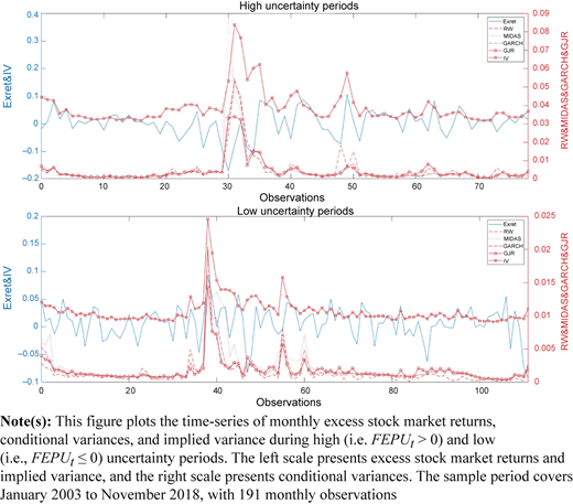
Figure 1 displays the time-series of monthly excess stock market returns, conditional variances and implied variance during high and low uncertainty periods, depending on the sign of FEPU. During low uncertainty periods, the conditional variances and implied variance tend to co-move with stock market returns. However, they move in the opposite direction of stock market returns during periods of high uncertainty. The correlations between stock market returns and variances are positive and statistically significant at the l% level during periods of low uncertainty. However, the correlations are negative and significant at the 1% or 5% levels in high uncertainty periods, except for the implied variance ^[8].

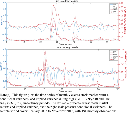
Figure 2 illustrates the time-series of monthly excess stock market returns, conditional variances and implied variance during high and low uncertainty periods, depending on the sign of FVOV. As shown in Figure 1, stock market returns tend to move closer to the conditional variances and implied variance during low uncertainty periods than during high uncertainty periods. While the correlations between stock market returns and variances during low uncertainty periods are positive and significant at the 5% or 10% levels, except for the case of the rolling window model, the correlations between them during high uncertainty periods are negative and significant at the 1% level except for the case of the implied variance ^[9]. For both FEPU and FVOV, the difference between the patterns of the correlations during high and low uncertainty periods suggests a positive mean–variance relationship in low uncertainty periods. Still, this relationship deteriorates in periods of high uncertainty.

The mean–variance relationship has been analyzed with the following regression:

where R_t+1 is the monthly excess stock market return, and Var_t(R_t+1) is the conditional variance or implied variance of the stock market returns for the next month t+1 based on conditional information at month t. To analyze the effect of uncertainty on this mean–variance relationship, we conduct the following two-regime equation:

where D_t is a dummy variable for the high uncertainty regime, the value of which equals 1 if month t is included in high uncertainty periods, and 0 otherwise ^[10, ^11]

Table 4 reports the coefficient estimates and t-statistics for the one-regime and two-regime equations. In the one-regime equation, the coefficient estimates (b) on the conditional variances estimated by the rolling window model and MIDAS are negative and significant at the 1% or 5% levels, as expected. Although insignificant, the coefficient estimates (b) on the conditional variances of GARCH(1,1) and GJR-GARCH(1,1) and implied variance are negative. The adjusted R²s of the one-regime equation range from −0.230% to 7.322%. Therefore, we confirm that a positive mean-variance tradeoff is reversed.

The results from the two-regime equation support our expectation that the mean-variance tradeoff varies with the degree of uncertainty. In low uncertainty periods, we find a significant positive tradeoff in models (1)-E, (2)-E, (2)-V, (3)-E, (3)-V, (4)-E, and 5-(E). Although the mean–variance relation is insignificant during low uncertainty periods in models (1)-V, (4)-V, and (5)-V, the coefficient estimates (b₁) are positive. In periods of high uncertainty, such a positive tradeoff is strongly undermined because the coefficient estimates (b₂) on the interaction term between D_t and the conditional variances or implied variance are negatively significant at the 1% or 5% levels. The adjusted R²s of the two-regime equation range from 1.261% to 12.482%, which is an improvement over those of the one-regime equation. The two-regime equation improvements in the adjusted R²s of FEPU, 3.855%p to 5.160%p, are always larger than those with FVOV, 0.924%p to 4.220%p.

Table 4 shows that considering uncertainty restores a positive mean–variance relationship across the four conditional variance models and model-free implied variance. Additionally, the impact of FEPU on the mean–variance relationship is larger than the impact of FVOV, and the results indicate that uncertainty has an important effect on the mean–variance relationship in stock markets. Therefore, we can confirm a varying mean–variance relationship depending on the level of uncertainty: The mean–variance relationship is significantly negative during high uncertainty periods, but a positive mean–variance relationship is observed during low uncertainty periods.

We perform an indirect test for the mean–variance relationship suggested by French et al. (1987) and Banerjee et al. (2007). Specifically, a regression is conducted to measure the relationship between future excess stock market returns and contemporaneous unexpected volatility innovations.

French et al. (1987) mention that if a larger conditional variance in the next month is predicted, the volatility innovation in the next month will decrease. Additionally, the variance for future periods will be revised upward. If there is a positive relationship between the risk premium and the predicted variance, the discount rate for future cash flows will increase. Thus, if cash flows are not affected, the current stock price, which is the discounted value of future cash flows from the firms, will decrease with a higher discount rate. Thus, there is a negative relationship between volatility innovation and future stock market returns if there is a positive relationship between conditional variance and future stock market returns.

Banerjee et al. (2007) develop a theory on the reactions of future returns to implied variance and implied variance shocks. If the price risk premium is positive and the implied variance positively predicts future realized variance, the level of implied variance and innovations of implied variance are positively related to future returns. For the VIX and S&P500 index excess returns, they provide empirical evidence that VIX is positively associated with 30-day and 60-day geometric returns on the S&P500 index. However, innovations in VIX are unrelated to future market returns.

Based on the above arguments for innovations on conditional variances and implied variance, we hypothesize a negative mean–innovation relationship in low uncertainty periods. Still, this relation is undermined in periods of high uncertainty. Additionally, we expect that innovations in VIX will positively impact future stock market returns during low uncertainty periods and negatively (or insignificantly) impact returns in periods of high uncertainty.

Before exploring these hypotheses, we first calculate the volatility innovation. Following French et al. (1987) and Yu and Yuan (2011), the volatility innovation in the rolling window model and MIDAS is calculated as the difference between the realized variance and the conditional variances:

Additionally, Yu and Yuan (2011) employ the monthly volatility innovations of GARCH(1,1) and GJR-GARCH(1,1) as the difference between conditional variances for month t+2 based on conditional information at month t+1 and conditional information at month t. Therefore, following Yu and Yuan (2011), we calculate the volatility innovations of GARCH(1,1) and GJR-GARCH(1,1) as follows:

Following Banerjee et al. (2007), we use the difference between the squared VIXs at month t and month t−1 as the innovations in the model-free implied variance:

Based on the estimated innovations on the conditional variances and implied variance, the return–innovation relationship is examined with the following regression:

where Var_t(R_t+1) is the conditional variance or implied variance of the stock market returns for the next month t+1 based on conditional information at month t, and Var(R_t+1)^u is the contemporaneous volatility innovation. To explore our hypotheses, we examine the following two-regime equation:

where D_t is a dummy variable for the high uncertainty regime, the value of which equals 1 if month t is included in high uncertainty periods.

Table 5 reports the results of the regression with volatility innovation. For the conditional variances of four models in Panels A to D, most of the coefficient estimates (e₂) on the interaction term between the volatility innovation and D_t are positively significant at the 1% or 5% levels, except for the volatility innovations of conditional variances estimated by GARCH(1,1) with D_t of FEPU and GJR-GARCH(1,1) with D_t of FVOV. Although the coefficient estimates (e) on the volatility innovation are always negatively significant, the magnitude of coefficient estimates (e₁) on the volatility innovation during low uncertainty periods becomes bigger than e in models (1) to (4). Among models with the conditional variances, the improvements in the adjusted R² range from 4.783%p to 9.281%p with D_t of FEPU and from 2.610%p to 4.606%p with D_t of FVOV. As shown in Table 4, the increments of the adjusted R² by considering FEPU are always larger than those by considering FVOV in models with the conditional variances.

In model (5) of Panel E, the relationship between future stock market returns and the innovation on the implied variance is significantly negative, which is inconsistent with the theory of Banerjee et al. (2007). Considering the effect of uncertainty, the coefficient estimates (e₂) on the interaction term between volatility innovation and D_t are negatively significant at the 1% level. Additionally, the coefficient estimates (e₁) on volatility innovation during low uncertainty periods are positively significant at the 1% or 10% levels. While the coefficient estimate (d) on the implied variance is insignificant in model (5), the coefficient estimates (d₁) on the implied variance during low uncertainty periods are positively significant at the 1% level in models (5)-E and (5)-V. In contrast to the results in models with the conditional variances, the improvement in the adjusted R² with exploiting FVOV is larger than that with exploiting FEPU.

To conclude, uncertainty impacts the relationship between future stock market returns and the expected variance, including the conditional variances and implied variance, and the relationship between future stock market returns and contemporaneous volatility innovations. We confirm that a negative relationship between the return and innovation of the conditional variance and a positive relationship between the return and the innovation of the implied variance are significant during low uncertainty periods. Conversely, uncertainty undermines these two relations in periods of high uncertainty. Such two-regime patterns provide indirect empirical evidence of the influence of uncertainty on the link between returns and volatility.

In this section, we check the robustness of our empirical results. In Section 4.1, we first replace the base assets to construct a mimicking factor for uncertainty. In Section 4.2, we analyze the mean–variance relation and the return–innovation relation after controlling for the effect of investor sentiment.

Lamont (2001) utilizes the return on four bond portfolios, eight industry-sorted stock portfolios, and the market portfolio for the stock market over the T-bill return as the base assets' returns for seven macroeconomic variables' mimicking factors. Ang, Hodrick, Xing, and Zhang (2006) use excess returns as the returns on the base assets to create a mimicking factor for innovation in VIX. Following them, we change the base assets from the Fama–French three factors to excess stock market returns (i.e. the market risk factor) ^[12].

Table 6 presents the regression results with the mimicking factor for uncertainty using excess stock market returns as the base asset's returns ^[13]. For the regressions of the mean–variance relationship, the coefficient estimates (b₂) on the interaction term between the variances and D_t are negatively significant at the 1% level, which undermines a positive mean–variance relationship. Although the coefficient estimates (b₁) on the variances are insignificant or significant at the 10% level, their sign is always positive, as expected. Compared with models (1) to (5) in Table 4, the changes of the adjusted R² range from 1.013%p to 4.252%p, which are always positive. Consistent with the results in Table 4, the results in models (1) to (5) of Table 6 indicate that the deteriorated mean–variance tradeoff is induced by uncertainty. Thus, considering uncertainty improves the explanatory power for the mean–variance relationship.

In the return–innovation relationship with four conditional variances, the coefficient estimates (e₂) on the interaction term between the volatility innovations and D_t are positively significant at the 1% or 5% levels, except for GJR-GARCH(1,1), in which the coefficient estimate (e₂) is insignificant. During low uncertainty periods, the coefficient estimates (e₁) on the innovations of the conditional variances are negatively significant at the 1% level, which is consistent with the empirical evidence in French et al. (1987). For the innovation of the implied variance, the coefficient estimates (e₂) are negatively significant at the 1% level, and the coefficient estimate (e₁) is positively significant at the 1% level. This positive sign of e₁ is consistent with Banerjee et al. (2007). The improvements in the adjusted R² range from 2.543%p to 10.479%p, compared with the adjusted R² in models (1) to (5) of Table 5. The results in models (1)-I to (5)-I of Table 6 also support our hypothesis that uncertainty weakens the return–innovation relationship. Consequently, a positive mean–variance relationship is undermined when uncertainty is high.

Yu and Yuan (2011) show the impact of investor sentiment on the mean–variance tradeoff in stock markets. They find empirical evidence that the expected stock market return is positively related to the conditional variance during low sentiment periods. Still, this positive relationship is weakened during high sentiment periods. These patterns are very similar to the results of this study. Therefore, in this subsection, the analyses in Tables 4 and 5 are repeated after controlling for the effect of investor sentiment on FEPU or FVOV. To control for the effect of investor sentiment, we perform the following regression:

where SENT_t−1 is Baker and Wurgler's (2006) investor sentiment index at month t−1 ^[14, ^15], and η_t (ν_t) is the residual FEPU (FVOV) in month t. D^I_t is a dummy variable for the high uncertainty regime based on FEPU (FVOV), the value of which equals 1 if η_t (ν_t) is positive. For equations (12) and (17), we replace D_t with D^I_t to analyze the effect of residual FEPU or residual FVOV on the mean–variance relationship and the return–innovation relationship.

Table 7 reports the regression results for the two-regime equation after controlling for the effect of investor sentiment. In models (1)-E to (5)-E, the coefficient estimates (b₂) on the interaction term between the conditional variances or the implied variance and D^I_t are negatively significant at the 1% level. Additionally, the coefficient estimates (b₁) on the conditional variances or implied variance are positively significant at the 1% level. In models (1)-V to (5)-V, the patterns of b₁ and b₂ are similar to those in models (1)-E to (5)-E. Furthermore, including D^I_t of the residual FEPU significantly improves the adjusted R², with a minimum and maximum increase of 4.462%p and 5.274%p, respectively. The improvements of the adjusted R² by exploiting the dummy variable of the residual FVOV range from 5.221%p to 6.500%p. These results in Table 7 are very similar to those of the two-regime mean–variance equations in Table 4.

In Table 8, we repeat the analysis for the return–innovation relationship in Table 5 with the dummy variables of the residual FEPU and residual FVOV. The results in Table 8 are similar to the two-regime return–innovation equations results with D_t in Table 5. The coefficient estimates (e₂) on the interaction term between the innovation on the conditional variances and D^I_t are positively significant at the 1% or 5% levels, except for GARCH(1,1), while the coefficient estimates (e₂) in the models with the innovation on the implied variance are negatively significant at the 1% level. During low uncertainty periods, the relationship between the return and volatility innovation is restored. Additionally, the adjusted R²s of all models in Table 8 are substantially improved by utilizing the dummy variable of uncertainty. Thus, these results confirm that including the dummy variable of uncertainty is valuable, regardless of controlling for the effect of investor sentiment on uncertainty.

This study examines the impact of uncertainty on the mean–variance tradeoff—high uncertainty undermines a positive tradeoff—which is further confirmed by the weakness of a negative relationship between contemporaneous innovations of conditional variances with stock market returns and a positive relationship of contemporaneous innovations of the implied variance with stock market returns during periods of high uncertainty. Additionally, our findings are robust to the change in the base assets used to construct the mimicking factor for uncertainty and the elimination of the influence of investor sentiment from uncertainty. Our empirical evidence is consistent with high ambiguity aversion and risk perception for investors, high cash flow risk and unfavorable investment opportunities, and the leverage effect during periods of high uncertainty.

Our paper extends the research on the asset pricing implications of option-implied uncertainty and risk. VOV and the implied variance have different information compared with EPU and the conditional variances, respectively. Therefore, we check the influence of VOV on the risk–return relationship and the relationship of the implied variance with stock market return depending on the level of uncertainty. Additionally, we provide a novel algorithm in which the information extracted from the options market, such as uncertainty and risk, exerts influence on the asset pricing model with rational investors and compensation for bearing risk.

Our study also suggests an additional perspective on portfolio management and policymaking. It is possible to apply uncertainty in making decisions regarding asset allocation and practical risk management. In addition, one policy implication of our findings is that regulators should require financial institutions to acknowledge the effect of uncertainty on risk measurement. For example, the impact of uncertainty can be considered when estimating value-at-risk (e.g. Xu et al., 2021), and the policymakers in the stock exchange should build the standard for the margin requirements based on value-at-risk estimates considering the level of uncertainty. Furthermore, researchers should reach a consensus on the measure of uncertainty. Although EPU and VOV show similar results in this study, the mechanisms of uncertainty impacting the risk–return relationship are different. We leave the further investigation to improve the measure of uncertainty to future research.

Funding: This work was supported by the Incheon National University Research Grant in 2021.