


The paper aims to enrich previous findings for an emerging banking industry such as Vietnam, reporting the difference between the parametric and nonparametric methods when measuring cost efficiency. The purpose of the study is to assess the consistency in issuing policies to improve the cost efficiency of Vietnamese commercial banks.
The cost efficiency of banks is assessed through the data envelopment analysis (DEA) and the stochastic frontier analysis (SFA). Next, five tests are conducted in succession to analyze the differences in cost efficiency measured by these two methods, including the distribution, the rankings, the identification of the best and worst banks, the time consistency and the determinants of efficiency frontier. The data are collected from the annual financial statements of Vietnamese banks during 2005–2017.
The results show that the cost efficiency obtained under the SFA models is more consistent than under the DEA models. However, the DEA-based efficiency scores are more similar in ranking order and stability over time. The inconsistency in efficiency characteristics under two different methods reminds policy makers and bank administrators to compare and select the appropriate efficiency frontier measure for each stage and specific economic conditions.
This paper shows the need to control for heterogeneity over banking groups and time as well as for random noise and outliers when measuring the cost efficiency.
1. Introduction
The efficiency of the banking industry has always been of particular concern to policymakers and researchers all over the world as banks play an extremely important role in the development prospects of each nation. That interest has been intensified over the last two decades, especially since the global financial crisis. When assessing the development prospects of banks, both researchers and managers rely on economic theories to measure and compare efficiency across banks. Efficiency measurement is an important reference for policymakers and market participants; however, Bauer et al. (1998, p. 88) show their concern when the efficiency scores of the banks are significantly different in most studies. Based on this, using the same set of data, the research is conducted to measure the efficiency of Vietnamese commercial banks in two different methods including the stochastic frontier analysis (SFA) and the data envelopment analysis (DEA). These are the two most commonly used efficient frontier measures in bank efficiency studies. The results of the two methods will then be analyzed and compared to make the most appropriate comments.
The Vietnamese banking industry provides an interesting background to evaluate cost efficiency of banks. The fledgling banking industry of Vietnam has continuously experienced important reforms. In particular, since joining the WTO, Vietnamese commercial banks have stepped up their restructuring, merger and acquisition (M&A) plans under a proposal proposed by the government. This program aims to improve the transparency, efficiency and competitiveness of the banking system. Therefore, an analysis of the change in the efficiency of banks is necessary to determine the success of the proposal. The effectiveness of restructuring policies in Vietnam will be an important reference basis for similar emerging banking industries.
The key issue leading to this study is the empirical performance of the efficiency frontier measures. The paper compares the results to find out whether there are significant differences in the DEA and SFA models across various samples. The main objective of this study is not to determine which approach is best for efficiency analysis, but it is important to find out the conflicting information provided by these two methods. Charnes et al. (1978) considered this approach a cross-checking method for consistency of efficiency measures. Through two different techniques, parametric and nonparametric, consistent results will be an important basis for policymakers and bank managers to be more confident in making decisions.
2. Literature review
DEA uses a linear programming technique to measure the relative efficiency of a set of similar decision-making units (DMUs), such as a set of same sector banks. DEA uses multiple inputs and outputs at the same time to determine efficiency scores which is used to evaluate DMUs. Through the linear programming, DEA compares each DMU with the others which have the same inputs and outputs. DEA defines an efficiency frontier as a linear set of the most efficient units. Therefore, DMUs being not on the frontier is ineffective. The DEA evaluates the relative efficiency of each DMU based on its distances to the efficient frontier. The farther away the DMUs are, the less effective they are.
Based on the concept of efficiency proposed by Farrell (1957), the DEA method had been first used by Charnes et al. (1978) which was studied under an input-oriented efficiency approach and the assumption of constant returns to scale (CRS). Later, Banker et al. (1984) proposed a variable returns to scale (VRS) model. These are two major DEA models that have been used extensively in many studies. Recent studies support the use of the DEA model with the VRS assumption because the former assumes that the CRS model is unrealistic and appropriate only when all banks operate on an optimal scale (McAllister and McManus, 1993; Mitchell and Onvural, 1996; Wheelock and Wilson, 1999; Sufian and Majid, 2008).
SFA is a very popular method for estimating the efficiency proposed by Aigner et al. (1977); Battese and Corra (1977) and Meeusen and van den Broeck (1977). This approach is developed from the idea that there are a number of factors that make DMUs not on the effective frontier and not entirely controlled by these DMUs. SFA allows the production functions to take into account the existence of errors when constructing the effective frontier. These errors are disentangled into random noise and inefficiency. The former represents the factors that affect the dependent variable but not observable, following a symmetric normal distribution. The latter represents inefficiency and often follows a truncated normal distribution (Berger and Humphrey, 1997, p. 15). The efficiency frontier of banks can be measured from the frontier cost or profit function estimations; however, this study uses only the cost function because of its popularity in the banking sector (Fries and Taci, 2005; Zhao et al., 2010; Mihai and Cristi, 2015).
Although the number of studies comparing the results between DEA and SFA is not much, these studies are still inconsistent. For example, the average efficiency scores measured by DEA and SFA are well-matched in Wadud and White (2000); Weill (2004) but not in Fiorentino et al. (2006); Delis et al. (2009) and Dong et al. (2014). On the other hand, Silva et al. (2017) assert that DEA and SFA provide similar conclusions about industry-level efficiency, but there is a distinction when efficiency is considered in each bank.
According to Bauer et al. (1998, p. 86), no method is the best for measuring efficiency. Thus, this study will analyze the consistency or antagonism from the results of two different cost-efficient frontier measures. The author performs a robust test of estimates from DEA and SFA based on distribution characteristics (mean, median, SD, minimum, maximum, skewness and kurtosis) efficiency rankings, time consistency, the identification of best or worst bank, the consistent correlations with traditionally used financial indicators and the determinants of efficiency scores by the time.
In Vietnam, a number of studies taken to compare efficiency among banks mainly use the nonparametric method – DEA (Ngo, 2010; Stewart et al., 2015). Recently, Nguyen et al. (2016) discovered similarities of the two methods when measuring the cost efficiency of Vietnamese banks according to each type of ownership and listing status. Wang et al. (2019) using loans as an output also had similar conclusions about the strong consistency of DEA and SFA in terms of cost efficiency. However, these studies only consider bank characteristics such as inputs or outputs when measuring the efficiency without taking into account the impact of macro factors. This study is conducted to fill that gap. In addition, the consistency over time of banks' cost efficiency measured by the two methods is further considered.
3. Methodology
3.1 The data envelopment analysis (DEA)
Cost efficiency refers to how a bank seeks to reduce input costs to the lowest level to create a certain amount of output. In other words, banks that adjust production technology must take into account the price of inputs in order to cut costs. Therefore, cost efficiency is calculated based on the combination of input-oriented technical efficiency and input–cost allocative efficiency. The cost efficiency model assuming VRS has form as follows:
subject to the following:
where are the number of bank; λ is a K*1 vector of constants; xi and yj are the vectors of inputs and outputs, respectively; is the amount of input that has minimalized the cost of the bank k at the given price wik and the certain amount of output yjk. The actual cost of bank k will be less than or equal to the (minimum) cost frontier . The optimal value of is found by solving the linear programming problem (1). The cost efficiency (CEk) of bank k is calculated by the ratio between the minimum cost and the actual cost below:
The cost efficiency examines how close the costs of bank are at the minimum (or the cost of a fully efficient bank) to produce a certain level of output at a given cost of input and technology. Thus, the cost efficiency (CE) shows that a bank can save (1−CE)*100% of the cost. Efficiency scores are also valid from 0 to 1 (or 100%). The cost efficiency score equals to 1 if the bank is the most cost effective or has the best cost savings in the sample; otherwise banks are cost ineffective if the efficiency score is less than 1. Banks with zero efficiency scores are considered to be the most wasteful banks. A bank is cost effective if it is both technically efficient and allocative efficient at the same time.
3.2 Stochastic frontier analysis (SFA)
When using the parametric method to estimate the cost efficiency of commercial banks, it is important first to consider the appropriate cost function. Accordingly, the trans log function is indicated because of its advantages over the Cobb–Douglas function and is most commonly used in bank efficiency studies (Kumbhakar and Lovell, 2003; Weill, 2013). The trans log function is highly flexible because it does not require too many constraints on alternatives between inputs, so it allows for the determination of scale efficiency at different output levels. In addition, the trans log function can impose parametric constraints (homogeneous conditions) to ensure that the estimation model adheres to the theoretical properties of the cost function. The trans log function provides the cost efficiency frontier model of the following form:
where TCit is the total cost (including interest expense and noninterest expense); is the outputs and is the price of the inputs; α, β, ϕ, μ, τ, θ, ρ and ω are estimated parameters; vit is the two-sided statistical noise component assumed to follow a standard normal distribution with a mean of zero, and uit is the inefficiency component of the composed error term according to the truncated normal distribution. T is a time trend that captures the impact of technological change leading to changes in production over time. T = 1 for the year 2005, T = 2 for 2006 … and T = 13 for 2017. Eqn (7) is estimated for each bank (i = 1,…, 34) over 13 years (t = 1,…, 13). Except for the T variable, all the other variables are given a natural logarithm. The coefficients in the cost function will be estimated using the maximum likelihood (ML) method.
The study assumes that banks have three output variables and three input prices based on the intermediate approach which regards banks as financial intermediaries, taking deposits and borrowing to provide loans and other assets. Accordingly, the assets may be considered as outputs whereas liabilities can be considered as inputs. Literature review on bank efficiency using the intermediary approach as well as the availability of Vietnamese data sources determines that deposits, labor cost and physical capital will be input factors used to generate outputs such as loans (Q1) and other earning assets (Q2) (Sealey and Lindley, 1977; Berger and Mester, 1997). Therefore, input prices include the ratio of interest expenses on total customer deposits (W1), the ratio of staff costs to total staff (W2) and the ratio of other operating expenses to total fixed assets (W3). On the other hand, recent bank studies have highlighted the significance of offbalance sheet items in almost all sectors of the bank, and their elimination may lead to underestimation of production and inaccurate estimates of bank performance (Casu and Girardone, 2006, p. 450). Therefore, the value of offbalance sheet items (Q3) is also considered to be an output factor.
Estimated results from the cost frontier model will be the basis for calculating the cost efficiency of each bank. It should be noted that the value of uit cannot be observed directly, but only the composite error can be observed. To solve this problem, it is possible to use conditional distributions to inefficiencies when estimating composite errors. In the case of truncated distribution, Battese and Coelli (1988) proposed an appropriate estimate of the cost inefficiency associated with the exponential function for the composite errors as follows:
where Φ(.) is the standard cumulative distribution function and . The value of γ must be between 0 and 1. If γ is equal to one, the deviation from the frontier is due to the cost inefficiency, while the zero value of γ indicates that the deviation is completely explained by statistical noise . The inefficiency measured by Eqn (8) is valid for [1, ∞) and is equal to one when the bank is fully effective. Accordingly, the cost efficiency score can be calculated as .
3.3 The model analyzes the determinants of cost efficiency
It is not necessary to explicitly explain the regression results to show the causal relationship between the determinants and efficiency of the bank; However, there may still be some important information demonstrating the consistency of the results by the two approaches in a regression framework. There are ten different determinants of bank efficiency to be analyzed as follows: (1) the size of the bank (LnTA) is represented by the logarithm of total assets; (2) the loan to deposit ratio (LTD) as a measure of liquidity of banks; (3) The cost to income ratio (CTI) represents the ability of banks to manage operating costs; (4) labor productivity (LP) is calculated by the ratio of total income to average total number of employees; (5) the nonperforming loan ratio (NLR) reflects the level of credit risk, an important factor that can affect the efficiency of banks; (6) the state's ownership structure is represented by a dummy variable which has the value of one if the bank has over 50% owned by the state and be equal to zero for the other banks; The two industry-specific determinants considered in the regression model are the competition and the growth rate of banking sector. (7) The competitive level of banks (Lerner) is represented by the Lerner index that is calculated by the difference between the output price and the marginal cost (Berger et al., 2009, p. 8); (8) the growth rate of the banking sector (BSD) is measured by the ratio of assets of banking sector to GDP; finally, banking efficiency is also analyzed under the influence of macroeconomic factors such as (9) inflation (INF) expressed by the CPI growth rate and (10) the economic growth rate (GDP). Data on bank characteristics are collected from Orbis Bank Focus, a database compiled by Fitch / Bureau Van Dijck that contains information about banks around the world, while macroeconomic data are provided by the World Bank.
Because the DEA method produces efficiency scores as censored dependent variables, the second-stage analysis of the DEA results uses a standard Tobit model, while for the SFA, the estimation method used is the POLS. The second-stage analysis is conducted using data in the three phases to reflect different periods of the business cycle. The first period of 2005–2007 is before the crisis, followed by the crisis and prerestructuring of the banking sector from 2008 to 2011, and the final phase represents the system restructuring period of 2012–2017.
3.4 Data
The study uses the annual panel data collected from 34 Vietnamese commercial banks, including 5 more 50% state-owned commercial banks (SOCBs), 26 joint stock commercial banks (JSCBs) and 3 joint venture banks (JVBs), provided by Orbis Bank Focus for the period 2005–2017. In addition, the macro data collected from the World Bank ensure reliability. Table 1 presents a summary of the descriptive statistics for the whole study period of the variables used in the models of bank efficiency.
Descriptive statistics of variables used in the DEA and SFA models
| Variables | Obs | Mean | Median | Sta. Dev. | Min | Max |
|---|---|---|---|---|---|---|
| Total cost (TC) | 410 | 7,967 | 3,032 | 12,276 | 7 | 67,613 |
| Loans (Q1) | 410 | 72,714 | 20,223 | 135,850 | 64 | 876,238 |
| Other earning assets (Q2) | 410 | 45,600 | 21,172 | 61,881 | 37 | 485,696 |
| Off-balance sheet items (Q3) | 410 | 18,110 | 2,672 | 37,532 | 0 | 336,905 |
| Deposits | 410 | 81,878 | 24,440 | 145,543 | 40 | 1,007,851 |
| Staff cost | 410 | 995 | 257 | 1,826 | 2 | 11,195 |
| Physical capital | 410 | 1,273 | 508 | 1,948 | 1 | 11,437 |
| Price of deposits (W1) | 410 | 0.094 | 0.079 | 0.052 | 0.023 | 0.393 |
| Price of staff (W2) | 410 | 0.143 | 0.134 | 0.075 | 0.008 | 0.415 |
| Price of physical capital (W3) | 410 | 1.053 | 0.729 | 1.269 | 0.052 | 16.227 |
In the vein of Fiorentino et al. (2006, p. 10), two important characteristics considered are developments over time and different banking group membership which affect SFA and DEA estimates. Therefore, efficiency frontiers are estimated not only for annual samples but also according to banking groups. The combination of the two characteristics is also considered for pooled samples. As a result, four samples exposed to SFA and DEA are respectively the following: (1) pooled over 13 years and three banking groups (All); (2) pooled banking pillars per year (years); (3) banking group specific frontiers pooled overall years (groups) and (4) separate banking pillar frontiers each year (both). Obviously, if these two characteristics affect efficiency scores measured by SFA and DEA the most, the differences between both measures in the last sample is expected to be the least (Fiorentino et al., 2006, p. 10).
4. Empirical results
4.1 Cost efficiency by the DEA method
The average cost efficiency of Vietnamese commercial banks obtained under the DEA method is shown in Table 2. The mean efficiency is not informative about the level of efficiency of a banking system but only a representation of the central tendency of the relative efficiencies.
The mean cost efficiency scores under the DEA method
| Years | All | Years | Groups | Both |
|---|---|---|---|---|
| 2005 | 0.6017 | 0.7833 | 0.6637 | 0.9102 |
| 2006 | 0.5524 | 0.3208 | 0.5992 | 0.8676 |
| 2007 | 0.5877 | 0.6758 | 0.6494 | 0.8295 |
| 2008 | 0.5066 | 0.7609 | 0.5778 | 0.9371 |
| 2009 | 0.5660 | 0.8844 | 0.6063 | 0.9497 |
| 2010 | 0.6512 | 0.8164 | 0.6677 | 0.8612 |
| 2011 | 0.7028 | 0.7547 | 0.7382 | 0.8920 |
| 2012 | 0.5783 | 0.7619 | 0.6298 | 0.9434 |
| 2013 | 0.5594 | 0.7874 | 0.6159 | 0.9290 |
| 2014 | 0.5677 | 0.7733 | 0.5850 | 0.9389 |
| 2015 | 0.5974 | 0.7907 | 0.6436 | 0.9324 |
| 2016 | 0.6612 | 0.7574 | 0.6842 | 0.8856 |
| 2017 | 0.7655 | 0.7645 | 0.7943 | 0.8940 |
| 2005–2017 | 0.6075 | 0.7409 | 0.6504 | 0.9054 |
It can be seen from the observation of the mean efficiency for each sample over year. During the study period (2005–2017), the average cost efficiency of the pooled banking sector is lowest at only 0.6075 compared to the different samples. Consistent estimates may be found in the sample of banking groups with the mean cost efficiency of 0.6504. The variability of DEA in both “All” and “Groups” models have significant similarity over time. On the other hand, the results of DEA estimates of separate banking groups each year provide the highest mean cost efficiency of 0.9054. In general, cost efficiency of the “Years” sample are lower than the “Both” sample but higher than the others, except for 2006; the cost efficiency from the “Years” model has dropped considerably to only 0.3208, much lower than the level of the other samples.
4.2 Cost efficiency by the SFA method
Table 3 presents the average of annual cost efficiency of Vietnamese banks estimated by the SFA method. For the pooled or separate banking groups over all years, the cost efficiency of banks has improved over time and is gradually approaching the optimal level. In general, the cost efficiency gap between these two samples is not large and tends to narrow over time. On the other hand, the cost efficiency of the SFA model for the models taking into account the effects of time-varying factors has significant variations throughout the study period. In the first phase, the “Years” model has higher cost efficiency than the two models without taking into account the effect of time. However, from 2013 onwards, the results tend to be the opposite. Meanwhile, the cost efficiency of banks by the “Both” model is also outperformed in the early stages but is gradually reaching the cost efficiency of the two models without the effect of time factor from 2012 to now.
The mean cost efficiency scores under the SFA method
| Years | All | Years | Groups | Both |
|---|---|---|---|---|
| 2005 | 0.7819 | 0.9163 | 0.7374 | 0.9981 |
| 2006 | 0.8356 | 0.8772 | 0.7992 | 0.9615 |
| 2007 | 0.8738 | 0.9981 | 0.8464 | 0.9331 |
| 2008 | 0.9060 | 0.9222 | 0.8880 | 0.9818 |
| 2009 | 0.9290 | 0.9368 | 0.9164 | 0.9577 |
| 2010 | 0.9468 | 0.9987 | 0.9380 | 0.9473 |
| 2011 | 0.9592 | 0.9988 | 0.9530 | 0.9988 |
| 2012 | 0.9704 | 0.9987 | 0.9662 | 0.9663 |
| 2013 | 0.9780 | 0.9177 | 0.9750 | 0.9745 |
| 2014 | 0.9833 | 0.9986 | 0.9813 | 0.9959 |
| 2015 | 0.9871 | 0.9396 | 0.9860 | 0.9849 |
| 2016 | 0.9901 | 0.9446 | 0.9897 | 0.9986 |
| 2017 | 0.9927 | 0.9366 | 0.9924 | 0.9956 |
| 2005–2017 | 0.9334 | 0.9526 | 0.9207 | 0.9765 |
In summary, the results obtained from both efficiency frontier models are strongly influenced by the time factor rather than the banking group, especially with respect to the SFA method. The mean cost efficiency of the two overall time models is highly consistent between the pooled banking groups and the individual banking groups for both the DEA and SFA approaches, while the differences in the models taking into account the effects of time variance are significant.
4.3 The comparisons of cost efficiency under DEA and SFA
4.3.1 Comparison of effective distribution
Table 4 shows a number of distributional characteristics of the cost efficiency obtained under the two methodologies. Overall, the mean cost efficiency according to SFA is higher than that for DEA. Moreover, when increasing the homogeneity of the sample, either methods react significantly differently. Minimizing the differences across banking groups and time leads to a significant increase in DEA scores from as low as 60.4%–90.6% in the most stratified sample while SFA mean efficiency increases only 5.5%. The inconsistency between two different efficiency measures is further illustrated by standard deviations, skewness and kurtosis of efficiency scores. Except for the sample stratified by both banking group and time, the SD of the SFA efficiency is generally lower than that of the DEA efficiency. This proves that the SFA efficiency measure is less volatile than DEA.
Descriptive statistics of cost efficiency according to SFA and DEA
| DEA | SFA | |||||||
|---|---|---|---|---|---|---|---|---|
| All | Years | Groups | Both | All | Years | Groups | Both | |
| Mean | 0.6044 | 0.7411 | 0.6476 | 0.906 | 0.9334 | 0.9535 | 0.9208 | 0.9755 |
| Median | 0.5665 | 0.79 | 0.605 | 1 | 0.9601 | 0.9972 | 0.9729 | 0.9979 |
| Std. Dev. | 0.1864 | 0.2586 | 0.2099 | 0.0203 | 0.0881 | 0.0811 | 0.1173 | 0.0632 |
| Min | 0.248 | 0.007 | 0.248 | 0.348 | 0.3585 | 0.5607 | 0.3226 | 0.5756 |
| Max | 1 | 1 | 1 | 1 | 0.9992 | 0.9999 | 0.9997 | 0.9999 |
| Skewness | 0.6548 | −0.8725 | 0.3583 | −1.439 | −2.5937 | −2.336 | −2.3087 | −3.7855 |
| Kurtosis | 2.5741 | 3.0915 | 1.9013 | 4.1522 | 11.666 | 8.1495 | 8.4157 | 18.1363 |
| Obs | 410 | 410 | 410 | 410 | 410 | 410 | 410 | 410 |
On the other hand, skewness in Table 4 shows that the cost efficiency under SFA is more asymmetric than those of DEA. The former is relatively close to one or closer to full efficiency than to full inefficiency. The former means that banks are relatively close to one or closer to full efficiency than to full inefficiency. Finally, the kurtosis of effective distribution according to the SFA method is much higher than that of the DEA. These results are consistent with Bauer et al. (1998) and Delis (2009).
In the DEA results in each year, a relatively large proportion of the banks is considered to be completely efficient as the efficiency frontier is established by a relatively large number of banks. Meanwhile, the efficiency frontier estimated by SFA is not a linear combination of the best performing observations but allows for measurement error. Figure 1 plots the efficiency scores obtained by SFA and DEA for all bank observations over time in turn for each sample.
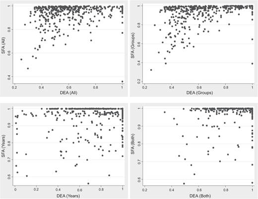
In summary, the comparison shows that there are some differences in distribution characteristics of the cost efficiency provided by the two different approaches. These differences may be due to different assumptions in each approach (Weill, 2004). However, these differences are not too serious a matter of deciding which method to encourage using. If different approaches can produce the same performance rankings, managers can still draw some rational policy conclusions from the cost efficiency scores analysis. Thus, the study then conducts an analysis of whether effective ranking orders according to different approaches are actually consistent.
4.3.2 Efficiency rankings
Table 5 describes the Spearman rank-order correlation coefficients across methodologies and samples. In general, rankings in the family of DEA method are more consistent than that of SFA. The correlations are on average higher for DEA (over 43%) compared to SFA (below 30%). However, the average of the coefficients between the two different families, shown in the lower left panel of Table 5, is only over 22%. Hence, two efficiency models generally do not rank banks in the same order, and thus the conclusions and policies drawn from these ranking orders may be contradictory.
The consistency of efficiency ranks across methods
| DEA | SFA | |||||||
|---|---|---|---|---|---|---|---|---|
| All | Years | Groups | Both | All | Years | Groups | Both | |
| DEA All | 1 | |||||||
| DEA Years | 0.2903*** | 1 | ||||||
| DEA Groups | 0.7961*** | 0.3018*** | 1 | |||||
| DEA Both | 0.4337*** | 0.3025*** | 0.4897*** | 1 | ||||
| SFA All | 0.2160*** | 0.1504*** | 0.2088*** | 0.1932*** | 1 | |||
| SFA Years | 0.2550*** | 0.2059*** | 0.2606*** | 0.1458*** | 0.2120*** | 1 | ||
| SFA Groups | 0.3023*** | 0.1828*** | 0.3735*** | 0.2002*** | 0.8655*** | 0.2691*** | 1 | |
| SFA Both | 0.2175*** | 0.1155** | 0.2642*** | 0.3213*** | 0.0886* | 0.1972*** | 0.1524*** | 1 |
| ROAA | 0.2049** | 0.2779*** | 0.1826* | −0.0546 | 0.2904*** | −0.0520 | 0.3097*** | −0.0688 |
| ROAE | 0.2749*** | 0.1162 | 0.2578*** | 0.1606 | 0.3260*** | −0.0401 | 0.2455*** | −0.0424 |
Note(s): (*, **, ***) correlation coefficients are significant at the level of 10%, 5% and 1%, respectively
An interesting result is that the rank correlation improves as both methods are used for the same samples of banking-group specific or both separate pillar and annually. The rank order correlations in these two cases are on average 35%. Thus, the same efficiency ranking of Vietnamese banks in the same order can be generally relied on DEA and SFA only for relative homogeneous samples. This has seemed to be a drawback of DEA because standard nonparametric methods do not take into account the heterogeneity and explain the difference between banks only as inefficiency (Fiorentino et al., 2006, p. 13). In addition, Table 5 also provides an inference of the relative advantages of group effects over time effects for the two methodologies passing from the fully pooled sample to the stratified subsamples. In particular, the group effect is severe than the time effect for DEA (reducing correlation from 100% to 29% instead of 79.6%), while for SFA (correlation reduces to 21.2% resp. 86.6%).
On the other hand, Table 5 also shows that the efficiency scores are not strongly correlated with the traditional accounting-based measures (return on average equity – ROAE and return on average asset – ROAA) for evaluating bank performance. This low magnitude is in line with almost previous researches (Bauer et al., 1998; Koetter, 2006; Fiorentino et al., 2006; Katharakis et al., 2014, and Silva et al., 2017). In addition, the all significant correlations are positive, indicating that the efficiency frontier measures contain additional information compared to the traditional performance ratios. It is noteworthy that the correlations between the SFA scores and traditional performance measures are in some cases larger than for DEA but also more varying across samples. Furthermore, much of the difference in performance rankings between traditional measures and cost efficiency are explained by the difference in samples according to banking pillars rather than time. Therefore, it is also important to control the systematic differences between various types of banks.
4.3.3 The consistency of the most and least efficient banks
Even if the ranking order of banks is inconsistent, the methods may still be meaningful for banking management purposes if they are consistent in determining which are the most and least efficient banks (Bauer et al., 1998, p. 105). This comparison is based on the idea of calculating the number of banks that are among the most (or least) effective banks not only under the DEA but also under the SFA. Table 6 presents the correspondence of extreme performers identified across both methodologies. The upper right triangle of the matrix in Table 6 reports for each pair of methods with various samples the proportions of banks that are identified simultaneously by both frontier efficiency methods to exhibit efficiency scores in the top 25%. For instance, 54.9% of the banks identified in the highest quarter by DEA in the pooled sample are also identified to be in the top 25% by SFA. If perfect correspondence gives a 100% level, a value of 54.9% indicates normal consistency.
Consistency of the most (or least) effective banks
| DEA | SFA | |||||||
|---|---|---|---|---|---|---|---|---|
| All | Years | Groups | Both | All | Years | Groups | Both | |
| DEA All | 1 | 0.7059 | 0.7745 | 0.6373 | 0.5490 | 0.5882 | 0.6667 | 0.5882 |
| DEA Years | 0.5784 | 1 | 0.6471 | 0.6863 | 0.5294 | 0.5882 | 0.6078 | 0.5294 |
| DEA Groups | 0.8922 | 0.5882 | 1 | 0.5980 | 0.4608 | 0.5000 | 0.6373 | 0.4412 |
| DEA Both | 0.7255 | 0.6373 | 0.7647 | 1 | 0.5882 | 0.7157 | 0.5196 | 0.6667 |
| SFA All | 0.5882 | 0.5882 | 0.6078 | 0.5588 | 1 | 0.7353 | 0.6176 | 0.6961 |
| SFA Years | 0.5980 | 0.6667 | 0.5784 | 0.5098 | 0.6765 | 1 | 0.5392 | 0.8235 |
| SFA Groups | 0.5686 | 0.6471 | 0.6176 | 0.5980 | 0.7647 | 0.6471 | 1 | 0.5000 |
| SFA Both | 0.6667 | 0.6471 | 0.7157 | 0.6667 | 0.6373 | 0.7451 | 0.7157 | 1 |
Note(s): This table shows the corresponding matrix of identified extremely efficient banks across methodologies. This matrix reports on each similarity ratio of a quarter of the lowest cost efficiency of banks determined by different techniques, while the correspondence between DEA and SFA when determining the top quarter is presented in the upper right triangle
In general, the correspondence between DEA and SFA for identifying bottom performers in the lower left triangle seems to be higher than for identifying top ones in the upper right of matrix. On average, the correlation of the least efficient banks identified by the two methods is about 61.4%, while the average correlation of the most effective banks is only 57.4%. Furthermore, there is no significant difference of the extreme performers taken care of within each method. The correspondence between the DEA samples is at the average of 69.8% for the worst and 67.5% for the best. In turn, the correspondence between the SFA samples is 69.8 and 65.2%. Therefore, the frontier efficiency techniques in identifying the worst banks are more consistent than in identifying the most effective banks.
Table 7 shows some of the most (or least) efficient banks by the two methods. These banks are ranked based on the average efficiency score of four samples for each method. There are three of the 34 banks listed with the highest efficiency by both methods – Bank for Investment and Development of Vietnam (BID), Vietnam Joint Stock Commercial Bank for Foreign Trade (VCB) and Tien Phong Commercial Joint Stock Bank (TPB). However, only one bank with the lowest efficiency appeared in both methods – National Citizen Commercial Joint Stock Bank (NCB). The bank with the highest average efficiency under DEA is Vietnam Bank for Agriculture and Rural Development (Agribank) while under SFA is Housing Bank of Mekong Delta (MHB). The least efficient bank under DEA is Nam A Commercial Joint Stock Bank (NamAbank) while under SFA is NCB.
The five most (or least) efficient banks
| Top 5 | Bottom 5 | ||
|---|---|---|---|
| DEA | SFA | DEA | SFA |
| Agribank (0.9474) | MHB (0.9888) | NamABank (0.5691) | NCB (0.8686) |
| BID (0.9282) | SCB (0.9858) | NCB (0.5775) | STB (0.8786) |
| VCB (0.9018) | TPB (0.9807) | KLB (0.5836) | ACB (0.8886) |
| CTG (0.9005) | VCB (0.9787) | SGB (0.5930) | PNB (0.8982) |
| TPB (0.8655) | BID (0.9784) | LPB (0.5990) | DAB (0.9129) |
4.3.4 The stability of efficiency frontier over time
For regulatory policy purposes, efficiency measurement methods will be more useful if estimated cost efficiency is relatively stable over time. Given the gradual volatility of the banking system in Vietnam, the effective ranking order of banks is expected to be unlikely to change significantly in the short term. A bank being currently very effective is not likely to become ineffective in the coming years; That is, it is likely that the bank could maintain its effectiveness over the next few years (Bauer et al., 1998, p. 106) unless there is a shock that is enough for the efficiency to fluctuate intensely in a short run. In order to test the stability of the efficiency over time, the average Spearman correlation coefficients in turn are calculated for each pair of yearly efficiencies for each of the different methodologies. Using data from 34 banks for 13 years (2005–2017), the 78 correlation coefficients for efficiency pairs corresponding to the k-year apart (k = 1, 2, …, 12) will be calculated for each method. Table 8 presents the average rank-order correlations for efficiency pairs by the number of years apart.
The stability of efficiency across k-year intervals
| k-year | 1 | 2 | 3 | 4 | 5 | 6 | 7 | 8 | 9 | 10 | 11 | 12 |
|---|---|---|---|---|---|---|---|---|---|---|---|---|
| DEA All | 0.740* | 0.569 | 0.509 | 0.418 | 0.366 | 0.349 | 0.376 | 0.296 | 0.268 | 0.207 | 0.116 | −0.036 |
| DEA Years | 0.541 | 0.431 | 0.370 | 0.270 | 0.235 | 0.199 | 0.067 | 0.071 | 0.053 | 0.025 | 0.021 | −0.317 |
| DEA Groups | 0.752 | 0.663 | 0.612 | 0.537 | 0.512 | 0.524 | 0.588 | 0.541 | 0.483 | 0.477 | 0.309 | 0.102 |
| DEA Both | 0.722 | 0.524 | 0.430 | 0.388 | 0.341 | 0.285 | 0.264 | 0.206 | 0.245 | 0.231 | 0.245 | 0.162 |
| SFA All | 1.000 | 1.000 | 0.999 | 0.999 | 0.998 | 0.997 | 0.997 | 0.996 | 0.995 | 0.993 | 0.991 | 0.989 |
| SFA Years | 0.235 | 0.125 | 0.029 | −0.042 | 0.018 | 0.029 | −0.021 | 0.050 | 0.019 | 0.162 | 0.024 | −0.305 |
| SFA Groups | 0.997 | 0.990 | 0.981 | 0.970 | 0.958 | 0.944 | 0.929 | 0.911 | 0.890 | 0.867 | 0.848 | 0.801 |
| SFA Both | 0.200 | 0.082 | 0.120 | 0.045 | 0.077 | 0.116 | 0.055 | 0.066 | 0.064 | 0.180 | 0.170 | 0.284 |
Note(s): *Each coefficient in this table represents the average correlation of the pairs of efficiency scores separated by k-years (k = 1, 2, …, 12) for each methodology across a 13-year period (2005–2017). Corresponding to each k-, the coefficient is reported as the mean of the (13-k) the correlation coefficients of the efficiency pairs with the interval of k-year. All correlation coefficients are significant at the 1% level
In general, the average correlation of efficiency is more consistent for all four samples according to DEA. In particular, the average correlation coefficient for the DEA banking group sample is highest at 0.752 when k = 1. However, the correlation coefficients tend to decrease gradually according to the magnitude of k. Most of the mean correlation coefficients for larger time distances are lower. Even in some cases, the coefficients are negative, indicating that the bank's ranking order has a considerable disturbance so that effective banks this year may no longer be effective after k years and vice versa. Thus, the efficiency frontier of Vietnamese commercial banks under the DEA method is only stable in the first 1–3 years. This shows that the efficiency rankings of banks have not changed significantly in the early years but tend to be different as the intervals increase. Relative changes in efficiency ranking over time are possible because the banking market is a competitive and dynamic environment (Fiorentino et al., 2006, p. 15).
On the other hand, the average rank-order correlations under the SFA method are very tight for the all and group samples where correlation coefficients are close to 1 in all years apart. However, for the year and both samples, the correlations are very loose when the average coefficients are close to zero. This shows the instability of the SFA method when measuring the overall efficiency of the banking system on a yearly basis. Accordingly, the SFA seems to be more appropriate to evaluate the effectiveness of each banking group.
4.3.5 The determinants of efficiency frontier
This section provides a second-stage regression analysis using the obtained cost efficiency as dependent variables to assess the importance of different determinants of bank efficiency. The results are useful in order to offer solutions to improve the cost efficiency of banks over time.
Table 9 reports the results of the second phase analysis. Although the relationship between bank size and efficiency is not consistent in the precrisis period, the DEA-based estimates provide evidence that the larger banks are more efficient in the latter two periods. On the contrary, the effect of liquidity on efficiency has been consistently achieved in the prerestructuring periods, but is not so clear afterward. The consistent positive effect of loan-to-deposit ratio shows that the banks holding liquid assets at a minimum are more efficient because loans generate a major source of interest income for banks. On the other hand, there is no clear evidence of the relationship between the ability to manage bank costs and the cost efficiency by the both approaches. However, in the only DEA model, banks with higher productivity will be more efficient. There is also evidence that nonperforming loans have a negative impact on bank efficiency in times of crisis. The type of bank ownership is clearly related to efficiency. Banks that are more than 50% owned by the state are more efficient than joint stock banks. This is true regardless of whether one considers the DEA or SFA models in all period. In addition, in only DEA-based estimates beyond the crisis period, competition actually has a significant negative impact on bank efficiency. A higher Lerner index or a lower level of competition shows the increase in efficiency. This result is consistent with the structure–conduct–performance (SCP) paradigm. The relationship between the sector growth and the bank efficiency is unclear in the previous periods, but the SFA-based estimates assert that the development of banking sector leads to banks being more efficient during the restructuring period. Finally, the diametrical opposite is also found in the relationships between macroeconomic factors and efficiency by two different models.
Second-stage regression results
| Dependent variable | DEA | SFA | ||||||
|---|---|---|---|---|---|---|---|---|
| All | Years | Groups | Both | All | Years | Groups | Both | |
| Estimation | (1) | (2) | (3) | (4) | (5) | (6) | (7) | (8) |
| 2005–2007 | ||||||||
| LnTA | 0.0278 | 0.0301 | −0.0008 | 0.1487*** | 0.0120* | −0.0273** | 0.0225** | −0.0190* |
| LTD | 0.3348*** | 0.0442 | 0.2441*** | 0.2816*** | 0.0050 | 0.0315 | 0.0129 | 0.0022 |
| CTI | 0.0127 | 0.0643 | −0.0055 | 0.0775 | 0.0060 | 0.0321* | 0.0129 | 0.0199 |
| LP | 0.0005 | 0.0952 | 0.0203 | 0.1011 | −0.0129 | −0.0111 | −0.0210 | 0.0209 |
| NLR | −0.0039 | 0.0023 | −0.0036 | −0.0142 | 0.0009 | 0.0031 | 0.0026 | −0.0017 |
| State | 0.1122** | 0.0132 | 0.3887*** | 0.0146 | −0.0406 | 0.0627* | 0.1395* | 0.0741** |
| Lerner | 0.5614*** | 0.2170 | 0.6286** | 0.9322 | −0.0514 | −0.0363 | 0.0144 | −0.0086 |
| BSD | −0.7324** | −4.3056*** | −0.6232 | −2.5801*** | 0.5533*** | 0.1789 | 0.6289*** | −0.3857* |
| INF | 1.7038** | 13.189*** | 2.1042* | 1.6688 | −0.4840*** | 2.1152 | −0.5733** | 0.3718 |
| GDP | Omitted | Omitted | Omitted | Omitted | Omitted | Omitted | Omitted | Omitted |
| 2008–2011 | ||||||||
| LnTA | 0.0848*** | −0.0096 | 0.0463*** | 0.0571* | −0.0087 | 0.0003 | −0.0118 | −0.0012 |
| LTD | 0.2929*** | 0.1347* | 0.2604*** | 0.3792*** | 0.0049 | 0.0446* | 0.0095 | 0.0537** |
| CTI | 0.0002 | 0.0237** | 0.0027 | 0.0034 | −0.0019* | 0.0018 | −0.0020 | −0.0021 |
| LP | 0.0288* | 0.1793*** | 0.0868*** | 0.0932** | 0.0064 | −0.0055 | 0.0081 | 0.0035 |
| NLR | −0.0073 | −0.0090 | −0.0078 | −0.0309** | −0.0027* | −0.0017 | −0.0040* | −0.0032 |
| State | 0.0081 | 0.2474*** | 0.2126*** | 0.2355** | 0.0284 | 0.0213 | 0.1175*** | 0.0430* |
| Lerner | −0.2077 | 0.1395 | 0.1437 | 0.4751 | 0.0148 | 0.0652 | 0.0353 | 0.0385 |
| BSD | 0.3769** | −1.1436*** | 0.0706 | −1.2230*** | 0.2915*** | 0.4207*** | 0.3601*** | 0.0825 |
| INF | 0.2649 | −2.5451*** | 0.1926 | −0.2370 | 0.1167** | 0.2453 | 0.1498* | 0.4721*** |
| GDP | −2.1399 | 8.1886* | −1.3029 | −2.0597 | −1.2713*** | 0.3068 | −1.5504*** | −2.9656** |
| 2012–2017 | ||||||||
| LnTA | 0.1207*** | −0.0505 | 0.0546*** | 0.0384* | −0.0005 | 0.0006 | −0.0032 | 0.0059 |
| LTD | 0.4575*** | 0.0067 | 0.4660*** | 0.4376*** | −0.0143*** | 0.0589* | −0.0110* | 0.0382* |
| CTI | −0.0038*** | −0.0034 | −0.0030* | −0.0043* | 0.0000 | −0.0008 | 0.0002* | −0.0003 |
| LP | 0.0056 | 0.1866*** | 0.0513*** | 0.0757*** | 0.0001 | 0.0075 | −0.0021 | −0.0112 |
| NLR | −0.0024 | −0.0064 | 0.0122 | 0.0004 | −0.0004 | −0.0060 | 0.0006 | −0.0033 |
| State | 0.0437 | 0.5157*** | 0.1384*** | 0.1461 | 0.0041 | 0.0140 | 0.0286*** | 0.0084 |
| Lerner | 0.2899** | 0.0941 | 0.5929*** | 0.8672*** | 0.0028 | 0.0298 | 0.0148 | 0.0126 |
| BSD | 0.1978 | 0.2379 | −0.0445 | −0.4928 | 0.0655*** | 0.3051** | 0.0762*** | 0.1944** |
| INF | 0.2692 | −2.9260 | 1.7787 | −2.0165 | −0.1829** | −2.8109*** | −0.2211* | −1.0878* |
| GDP | −0.9704 | −6.4634 | 12.108 | −3.9897 | −0.5974 | −17.846*** | −0.6544 | −6.8068* |
Note(s): (*, **, ***) correlation coefficients are significant at the level of 1%, 5% and 10%
5. Conclusion
The study is conducted to compare the cost efficiency of Vietnamese commercial banks by the DEA and SFA methods to assess the similarity in the issuance of policies. The results show that the SFA models estimate higher efficiency scores and less significant variability than the DEA models. Moreover, the mean cost efficiency calculated for each banking group is lower than for that taking into account the effect of time factor on both approaches. Fiorentino et al. (2006, p. 17) interprets this result as the parametric nature of SFA found to be less sensitive to external factors due to measurement error. Meanwhile, because DEA uses a deterministic boundary to full efficient banks, this method is much more sensitive to the choice of the banks included in the sample. When evaluating the relative efficiency of the three pillar system of Vietnamese banks, higher heterogeneity in the data leads to low mean efficiency because other factors affecting cost efficiency as technical fluctuations over time are taken into account. Subsequently, the sensitivity of the average sector efficiency levels is estimated by setting increasingly homogeneous samples across years and banking groups. The results show that the SFA and DEA measures provide the highest scores when comparing only banks of one group per year. Therefore, DEA should be used with care because there is clearly possibility to believe the dominance of measurement errors.
On the other hand, the comparison shows that there are some differences in the distribution characteristics and the ranking order correlation of the efficiency scores provided by two different methods in this study. The analysis of bank rankings across methodologies and samples does not show evidence that both measures exhibit a high correlation in rank order. However, the rankings in the DEA family are more appropriate than SFA. This shows the importance of checking the robustness of the efficiency ranking using different methods.
For the stability of efficiency over time, it is clear that ongoing fluctuations in the industry over the past decade, such as restructuring and increased competition, have had a significant impact on the efficiency rankings over the years. The DEA-based models seem to show a more consistent variation over time, while the SFA method only provides the stable rankings when only applying samples without the time effect. Thus, when assessing the efficiency frontier of banks, it is necessary to consider the change over time that is due to many causes.
The two methods also show a fairly high consistency in identifying the most efficient and least efficient banks for all samples as all correlation coefficients are greater than 0.5. In addition, the results also show that the obtained cost efficiency has a positive but not significant correlation with traditional accounting-based measures. This indicates that efficiency measures contain additional information compared to traditional performance ratios. Finally, an analysis of the development of the effectiveness of Vietnamese banks over time also poses many challenges to address, such as increasing bank size, enhancing labor productivity, reducing nonperforming loans, control of competition and inflation.
Because banks have different operating periods, the research data are unbalanced. There are a few banks that only provide data for eight years, while the maximum study period of other banks is up to 13 years. This study is limited not only to the number of observations in the sample but also to the scope of only one country. Therefore, further studies may consider using a larger sample set of countries and extending the study period to provide a more comprehensive analysis of the cost efficiency of banks in emerging countries.

