


The study’s first aim is to estimate the scale of working poverty using a nationwide household survey. The second aim is to answer the following research questions: is working enough to escape poverty, and what are the determinants of working poverty?
The focus is on working people in Indonesia who have per capita household expenditure below the provincial poverty line. The determinant analysis used logistic regression on the first quarter of 2013 Susenas microdata.
The study found that the scale of the working poverty problem is equivalent to the scale of the poverty, although the in-work poverty rate is lower than the poverty rate in all provinces. The logistic regression results conclude that the three factors, namely individual-level, employment-related and household-level variables, have significant contributions to the incidence of the working poor in Indonesia.
Some practical implications for reducing the incidence of working poverty are increasing labor earnings through productivity growth and improving workers' skills, encouraging the labor participation of the poor and reducing precarious work. This study also suggests the need to continue assisting the working poor, particularly by increasing access to financial credit.
Research aimed at studying working poverty in Indonesia in the peer-reviewed literature is rare until now based on the authors' search. This study will fill the gap and provoke further research on working poverty in Indonesia.
1. Introduction
Employment and poverty are closely related and a part of the poverty reduction strategy. The employment-reducing poverty strategy starts with the job creation to employ the poor. From the supply side, improving education and skill promote employability simultaneously by creating an efficient labor market (Karnani, 2011). However, these are not necessarily enough to reduce the risk of poverty if the wages or income received are lower than the standard of living (Cheung and Chou, 2016; Feder and Yu, 2019; ILO, 2019; Fibaek, 2021). To escape poverty, poor people must have decent and more productive work to increase their income, even though the relationship between low-paid employment and poverty is not straightforward (Feder and Yu, 2019).
Studies on working poverty have recently been growing in the last decade, especially in developed countries (Lohmann, 2009; Brady et al., 2010; Herman, 2014; Cheung and Chou, 2016; Thiede et al., 2016; Lyon, 2018; Filandri et al., 2020). The results show that working poverty is fundamental to the fight against poverty. However, the working poor is found both in developed and developing countries (Gangopadhyay et al., 2014; Feder and Yu, 2019; Fibaek, 2021). Even in developing countries, the proportion of working poor is higher (ILO, 2019).
According to the International Labour Organization (ILO) estimate, 21% of all employed persons in 2018 around the world live in poverty (ILO, 2019). In Indonesia, the working poverty rate calculated based on the national poverty line was 14.4% in 2010. Although the percentage has decreased significantly compared to 1996, the absolute number is not much different, around 16 million people (ILO, 2011). Meanwhile, the number of poor people in Indonesia in the same year (2010), based on the National Statistics Office Report, was 31.02 million people. This large number of working poor required more concern in poverty alleviation in Indonesia. There is no unemployment benefit in Indonesia, so every adult has to work regardless of earnings.
Research on working poverty in Indonesia in the peer-reviewed literature is rare until now based on the authors' search. However, knowledge about the working poverty associate factors is urgent for designing and implementing poverty alleviation policies. This paper will fill the gap and provoke further research on working poverty in Indonesia. The primary focus is the working people but has per capita household expenditure below the provincial poverty line. The first aim is to estimate the scale of working poverty using a nationwide household survey. The second aim is to answer the research questions: Is working enough to escape poverty, and what are the determinants of working poverty?
2. Conceptual framework and literature review
Three main theories explain poverty causes are behavioral, structural and political (Brady, 2019). The behavioral theory views poverty from individual behavior driven by culture. The structural view focuses on the demographic and economic aspects. At the same time, the political theory states that power and institutions make policies that cause poverty. From the structural context, demographics and employment can directly cause poverty or indirectly influence behavior change.
As employment is fundamental to poverty reduction, the factors affecting the incidence of working poverty are noteworthy to explore in-depth. Past research has identified some factors causing working poverty at the macro- and micro-levels. At the macro-level, economic performance, labor market institutions and welfare regimes affect the working poverty incidence (Lohmann, 2009; Crettaz, 2011; Cheung and Chou, 2016; Levanon et al., 2019). The micro-level-factors comprise individual, household and employment-related factors (Cheung and Chou, 2016; Lohmann, 2018; Levanon et al., 2019). The individual-level factors are age, sex, education and marital status, while the household-level factors are the number of earners, dependents and household access to financial credits. The last is the employment-related factors, for example, the job sector, working hours and employment status.
Brady et al. (2010) examined working poverty in 18 countries using the Luxembourg Income Survey. They found that working poor did not reflect the overall picture of poverty, but other factors include demographic characteristics and welfare generosity. Levanon et al. (2019) also found the influence of these demographic characteristics in their studies in Germany and Israel. Bodea and Herman (2014) found that the primary determinant of working poverty in Romania relates to vulnerability in employment and precariousness. These determinants include self-employment, low wage and low education level. Herman (2014) found the same factor of working poverty for other European countries. In Germany, low education workers are more at risk of poverty, while in the United Kingdom (UK), old-age workers are more at risk Giesselmann (2015).
Linneker and Will (2016) highlighted the effect of living wages on reducing working poverty in the UK, while Filandri et al. (2020) emphasized the impact of job intensity and job stability on working poverty in Italy. There was a significant effect of low wages on working poverty in the USA (Lyon, 2018), as well as in Hong Kong (Cheung and Chou, 2016), South Africa (Feder and Yu, 2019) and Kenya (Fibaek, 2021). Working poverty is also related to material deprivation (Cheung et al., 2019) and political inclusion (Marinova, 2020). The political aspect of poverty reduction is crucial because power and institutions are responsible for making poverty policies (Brady, 2019).
The factors above cause working poor through three mechanisms: (1) low earnings, (2) low labor participation and (3) high household burden (Crettaz, 2011; Crettaz and Bonoli, 2011; Cheung and Chou, 2016). Macro-level and individual-level factors influence low earnings and low labor participation, while job characteristics only affect the earnings received by individual workers. Finally, household-level factors affect labor participation and household burden (Figure 1).
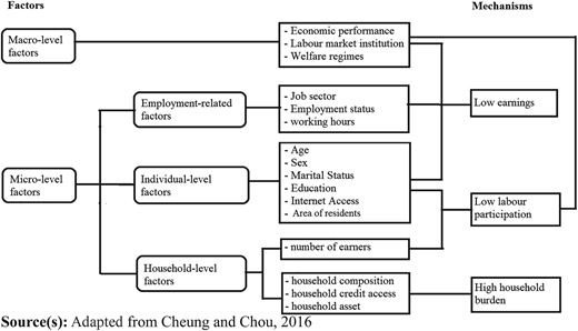
The low earnings mechanism comes from macrolevel factors: macroeconomic performance, labor market institutions and welfare regimes (Lohmann, 2009; Crettaz, 2011). In a good macroeconomic performance, the productivity grows so that the companies' ability to pay higher wages increases. The combination of globalization, industrialization and technological change promotes economic efficiency and increases productivity. In line with that, the government could implement policies on improving the quality of labor through education and training to increase labor productivity. Despite companies' compliance, the Indonesian government implements a minimum wage policy to protect workers.
The microlevel factors that influence low earnings are individual-level factors and employment-related factors. Individual characteristics, such as age and education, are related to ability, skill and experience that finally affect earnings (Milanovic, 2006; Baffour, 2015; Franzini and Raitano, 2019). The employment characteristics that reflect the current work situation also determine income. Informal workers, for instance, usually have low earnings (Nezhyvenko and Adair, 2017), as well as other precarious workers. Informality is also subject to more volatile low earnings in developing worlds (Gomes et al., 2020). Bodea and Herman (2014) also supported the relationship between precariousness and working poverty in their research in Romania.
The second mechanism is low labor participation contributed by macrolevel and microlevel factors (individual and household-level factors). From a macroperspective, the economic structure often restrains women's opportunity to work in developing countries (Klasen, 2018). At the micro-level, it is clear that individual demographic characteristics, such as age, education and gender, as well as household composition, have a powerful influence on a person's willingness to work. The labor market institution and the demographic variables simultaneously determine employment structure (Bertola et al., 2007).
The last mechanism is the high household burden caused by high household needs but limited household resources. Previous researchers, such as Brady et al. (2010) and Cheung and Chou (2016), have disclosed the high household burden as the working poverty cause. The unfulfillment of basic needs is the core of poverty. In Indonesia, preventing the increase of poverty during crises, the government helps vulnerable households with financial credit or other social aid (Dhanani and Islam, 2002).
3. Data and methods
3.1 Data
The data used in this paper are from a nationwide household survey – National Socio-economic Survey (Survei Sosial Ekonomi Nasional – Susenas). Instead of using the National Labour Force Survey (Survei Angkatan Kerja Nasional – Sakernas), Susenas is more appropriate because it collects employment, other households’ socioeconomic and household expenditure. Thus, Susenas can link the poverty status with the employment status of household members. It is difficult to perform a micro-analysis of working poverty using Sakernas data because of the absence of household poverty status in Sakernas microdata. However, the limitation of using Susenas data is that there are relatively few questions related to employment.
This paper uses the first quarter of 2013 Susenas microdata collected in March by BPS-Statistics Indonesia. Besides the broad socioeconomic aspects covered, Susenas (2013) has a large sample size of over 75 thousand households per quarter and representatives up to the provincial level. The worker earnings were asked in Susenas, 2013, even though omitted in the next Susenas, this paper preferably used the 2013 Susenas, not the latest Susenas.
3.2 Methods
The term working poverty consists of two concepts: working and poverty. The working concept used in this paper refers to BPS-Statistics Indonesia in both Sakernas and Susenas. Officially, BPS defined a working (or an employed) person as a person aged 15 years or older who have worked for pay or profit for at least one consecutive hour during a week or has a job but is absent because of holidays, sick leave or others (BPS, 2020b). Meanwhile, the poverty definition is a monetary approach. Poor people cannot meet the minimum needs equivalent to 2,100 kcal per capita basic food needs per day and the minimum nonfood needs (BPS, 2019).
Working poor is a status of a working person who lives in a poor household. This definition combines the labor market status of an individual with the poverty status. Thus, the working poverty rate is the proportion of the working poor to the total working population age of 15 years and over. This paper uses each provincial poverty 2013 applied to the 2013 Susenas microdata to determine if a household is poor or not.
The method of analysis in this paper is as follows: first, the differences in working poverty rate between provinces and socioeconomic factors using descriptive analysis and chi-square bivariate analysis to measure their association further. The next step is employing logistic regression methods to determine factors affecting working poverty in Indonesia. Following Hosmer et al. (2013), the logistic regression model is formulated as follows:
where y is the dependent variable, represents the conditional mean of y given X, X is the vector of the independent variables (X1, X1, …, Xp)’, and is the error term binomially distributed with a mean zero and variance . in equation (1) above is transformed using the following logit transformation so that the regression model has desirable properties of linear regression:
The parameters' estimation method of the logistic regression model uses maximum likelihood estimation, while the computation process in this paper utilizes STATA 16.0 software.
One advantage of logistic regression is a meaningful interpretation using the odds ratio. The odds ratio is the ratio of the odds of the one category of the independent variable to the odds of the reference category. The odds ratio approximates how likely (in terms of odds) the outcome variable is happening in one group of independent variables compared to the reference group (Hosmer et al., 2013).
The dependent variable used here is the poverty status of an individual worker. The independent variables comprise individual-level, employment-related, household-level and location-related variables. Table 1 presents the descriptions of all variables used in this paper. Variables with over two categories in the regression model changed into two or more dummy variables with the reference category 0.
Description of the variables
| Variables | Description |
|---|---|
| Dependent variable | |
| WPOOR | Poverty status of worker (0 = not poor, 1 = poor) |
| Individual-level variables | |
| AGE | Age of worker (0 = 15–39 years, 1 = 40–59 years, 2 = 60 years or older) |
| SEX | Sex of worker (0 = female, 1 = male) |
| MARITAL | Marital status of worker (1 = married, 0 = others) |
| EDUC | Education level of worker (0 = primary school or no school, 1 = secondary school, 2 = high school, 3 = college or university) |
| INTERNET | Internet access of worker (0 = no access, 1 = has access) |
| Employment-related variables | |
| SECTOR | Primary job sector of worker (0 = agriculture, 1 = manufacturing, 2 = services) |
| HOURS | Weekly working hours of worker (0 = less than 35 h per week, 1 = 35 h or more) |
| STATUS | Employment status of worker (0 = employees, 1 = casual workers, 2 = own-account workers, 3 = contributing family workers or unpaid workers, 4 = employers) |
| EARNINGS | Labor individual earnings (1 = lower than provincial minimum wage, 0 = above provincial minimum wage) |
| Household-level variables | |
| PNWOK | The proportion of working to the total household member |
| ASSET | Ownership of household assets (0 = no asset, 1 = has asset) |
| CREDIT | Household access to microfinance (0 = no access, 1 = has access) |
| Location-related variables | |
| UR | Urban–rural classification (0 = rural, 1 = urban) |
| PROV | Province (0 = Yogyakarta) |
This paper uses access to microcredit as one of the independent variables, in contrast to Ahmed et al. (2016), which includes the variable availability of financial institutions in the regression model. Anindyntha et al. (2021) found that only two financial inclusion variables affect poverty reduction in Indonesia: financial access and financial usage. At the same time, the availability of financial institutions has no significant effect on poverty. We also use individual earnings as a categorical independent variable in the model to see the influence of minimum wage on poverty. Although applying the minimum wage reduces poverty in developing countries (Gindling, 2018), researchers in Indonesia reveal different results from one another. This variable is not identical with poverty status because household poverty status is determined based on household expenditure.
4. Empirical findings
4.1 Descriptive and bivariate analysis
Table 2 compares the working poverty rate between categories or groups of the individual-level, employment-related and household-level variables. There are strong associations between the in-work poverty rate and almost all individual-level variables, except the sex of the worker. In terms of age, the lowest rate based on age is 40–59, the mature period in career or job. The married persons are worse off than the not married or divorced, perhaps because of more dependents. Workers who live in urban areas or have Internet access or higher education have working poverty at a lower rate. On the other hand, there is no different working poverty rate between men and women.
Working poverty rate, poverty headcount ratio and chi-square measure of association by variables
| Variables | Poverty headcount ratio (%) | Working poverty rate (%) | Chi-square measure of association | |
|---|---|---|---|---|
| Statistics | p-value | |||
| Overall | 10.61 | |||
| Age of worker | 82.90 | 0.00 | ||
| 15–39 years | 11.30 | 11.25 | ||
| 40–59 years | 9.44 | 9.66 | ||
| >= 60 years or above | 11.57 | 11.22 | ||
| Sex of worker | 1.49 | 0.22 | ||
| Male | 12.36 | 10.52 | ||
| Female | 12.41 | 10.73 | ||
| Marital status | 6.28 | 0.01 | ||
| Married | 13.82 | 10.73 | ||
| Others | 10.77 | 10.23 | ||
| Urban–rural | 1,500.00 | 0.00 | ||
| Urban | 7.95 | 6.62 | ||
| Rural | 15.74 | 13.43 | ||
| Education | 3,400.00 | 0.00 | ||
| No school or primary school | 15.58 | 15.01 | ||
| Secondary school | 9.56 | 9.77 | ||
| High school | 5.37 | 5.24 | ||
| College/university | 1.18 | 1.11 | ||
| Internet access | 1,500.00 | 0.00 | ||
| No Internet access | 13.33 | 11.82 | ||
| Has Internet access | 2.71 | 1.59 | ||
| Worker earnings | 2,200.00 | 0.00 | ||
| < Provincial minimum wage | 12.53 | |||
| >= Provincial minimum wage | 2.18 | |||
| Primary job sector | 4,200.00 | 0.00 | ||
| Agriculture | 16.75 | |||
| Manufacturing | 8.84 | |||
| Services | 4.80 | |||
| Weekly hours of work | 551.52 | 0.00 | ||
| < 35 h | 13.32 | |||
| >= 35 h | 9.12 | |||
| Employment status | 2,800.00 | 0.00 | ||
| Employees | 5.37 | |||
| Casual workers | 15.75 | |||
| Own-account workers | 11.38 | |||
| Contributing family workers | 17.06 | |||
| Employers | 3.79 | |||
| Household asset ownership | 6,400.00 | 0.00 | ||
| No asset | 27.87 | 24.06 | ||
| Has asset | 8.44 | 7.14 | ||
| Household access to microfinance | 344.15 | 0.00 | ||
| No access | 13.00 | 11.19 | ||
| Has access | 7.53 | 6.26 | ||
| The average proportion of working household members | Poor: 0.50N on-poor: 0.60 | |||
Note(s): Number of observations: 129,257
Source(s): authors' calculation without sampling weight
All the employment-related variables have strong associations with working poverty, implying the very importance of employment characteristics on the poverty status of workers. Workers who receive earnings above the provincial minimum wage or work over 35 h per week have a much lower level of working poverty. Otherwise, workers in the agricultural sector have the highest level of working poverty than other sectors. Based on employment status, workers with an increased working poverty rate contribute to family workers, casual workers and own-account workers.
All three variables at the household level have a strong relationship with working poverty. The working poverty rate for families having assets is much lower because households use their assets, including productive assets, as business capital to combat poverty. Financial credit access also results in a much lower incidence of poverty than those with no access. The poor households also have a lower proportion of working members than the nonpoor, as the number of working members prevents them from becoming poor.
This paper also compares the poverty and working poverty rate among provinces (Table 2 and Figure 2). A high poverty rate province also has a high in-work poverty rate and vice versa. However, the working poverty rates are lower than the poverty rates for all areas in Indonesia. It means that the scale of the in-work poverty problem is almost equivalent to the scale of poverty. However, having a job at least reduces the probability of being poor because working gives people the opportunity to escape poverty. This finding supports the argument that solving working poverty problems is strongly contributes to reducing the poverty rate.
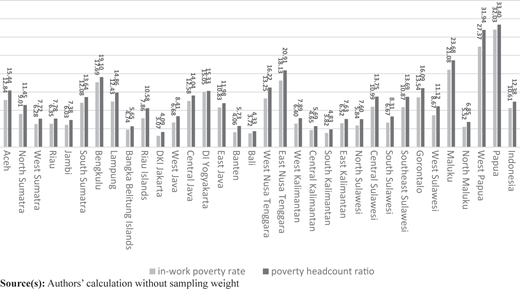
It is curious to compare the working poverty rate and the poverty rate because the differences are higher in some provinces. For example, we found the higher difference in Maluku, West Papua, West Nusa Tenggara, East Nusa Tenggara, Riau Islands, Southeast Sulawesi and Aceh. Although we do not want to discuss the causes of the variations of the difference, some of the above provinces, based on related data, have relatively high open unemployment rates (BPS, 2014b). A higher proportion of unemployed people may trigger this higher difference.
4.2 Determinants of working poverty
To answer the primary research questions, we perform logistic regression. The aim is to verify the three groups of microlevel variables expected as determinants of working poverty in Indonesia. Because several variables may interact, the regression model includes the interaction of variables. Table 3 below presents the results obtained from logistic regression.
Logistic regression estimates of the determinants of working poverty
| Variables | Odds ratio | Standard error | |z| | p-value |
|---|---|---|---|---|
| Individual-level variables | ||||
| Age | ||||
| 40–59 years | 0.89 | 0.02 | 4.56 | 0.00** |
| 60 years or older | 0.97 | 0.04 | 0.83 | 0.41 |
| Sex | ||||
| Male | 1.07 | 0.06 | 1.20 | 0.23 |
| Marital | ||||
| Married | 0.83 | 0.02 | 6.99 | 0.00** |
| Educ | ||||
| Secondary school | 0.82 | 0.04 | 4.17 | 0.00** |
| High school | 0.66 | 0.04 | 7.63 | 0.00** |
| College/university | 0.49 | 0.07 | 4.95 | 0.00** |
| Internet | ||||
| Has Internet access | 0.43 | 0.03 | 11.81 | 0.00** |
| Employment-related variables | ||||
| Earnings | ||||
| ≥ Provincial minimum wage | 0.21 | 0.03 | 10.76 | 0.00** |
| Sector | ||||
| Manufacturing | 0.81 | 0.05 | 3.19 | 0.00** |
| Services | 0.62 | 0.03 | 9.08 | 0.00** |
| Status | ||||
| Casual workers | 1.09 | 0.07 | 1.31 | 0.19 |
| Own-account workers | 0.76 | 0.04 | 4.99 | 0.00** |
| Contributing family workers | 1.23 | 0.07 | 3.93 | 0.00** |
| Employers | 0.30 | 0.06 | 5.65 | 0.00** |
| Hours | ||||
| 35 h per week or more | 1.07 | 0.03 | 2.39 | 0.02* |
| Household-level variables | ||||
| PNWOK | 0.04 | 0.00 | 59.65 | 0.00** |
| Asset | ||||
| Has assets | 0.34 | 0.01 | 45.33 | 0.00** |
| Credit | ||||
| Has credit access | 0.63 | 0.02 | 12.66 | 0.00** |
| Location-related variables | ||||
| UR | ||||
| Urban | 1.36 | 0.06 | 6.66 | 0.00** |
| PROV | ||||
| Aceh | 0.41 | 0.04 | 9.94 | 0.00** |
| North Sumatra | 0.23 | 0.02 | 17.17 | 0.00** |
| West Sumatra | 0.20 | 0.02 | 15.98 | 0.00** |
| Riau | 0.23 | 0.02 | 13.78 | 0.00** |
| Jambi | 0.20 | 0.02 | 14.49 | 0.00** |
| South Sumatra | 0.40 | 0.04 | 10.25 | 0.00** |
| Bengkulu | 0.63 | 0.06 | 4.79 | 0.00** |
| Lampung | 0.44 | 0.04 | 9.09 | 0.00** |
| Bangka Belitung Islands | 0.20 | 0.03 | 11.23 | 0.00** |
| Riau Islands | 0.46 | 0.06 | 6.19 | 0.00** |
| DKI Jakarta | 0.19 | 0.03 | 10.79 | 0.00** |
| West Java | 0.20 | 0.02 | 18.18 | 0.00** |
| Central Java | 0.56 | 0.04 | 7.25 | 0.00** |
| East Java | 0.47 | 0.04 | 9.33 | 0.00** |
| Banten | 0.14 | 0.02 | 15.78 | 0.00** |
| Bali | 0.19 | 0.02 | 13.44 | 0.00** |
| West Nusa Tenggara | 0.32 | 0.03 | 11.60 | 0.00** |
| East Nusa Tenggara | 0.25 | 0.02 | 15.98 | 0.00** |
| West Kalimantan | 0.19 | 0.02 | 16.03 | 0.00** |
| Central Kalimantan | 0.17 | 0.02 | 15.49 | 0.00** |
| South Kalimantan | 0.15 | 0.02 | 15.58 | 0.00** |
| East Kalimantan | 0.28 | 0.03 | 11.91 | 0.00** |
| North Sulawesi | 0.13 | 0.02 | 17.76 | 0.00** |
| Central Sulawesi | 0.29 | 0.03 | 12.27 | 0.00** |
| South Sulawesi | 0.16 | 0.01 | 19.72 | 0.00** |
| Southeast Sulawesi | 0.31 | 0.03 | 11.54 | 0.00** |
| Gorontalo | 0.34 | 0.04 | 9.24 | 0.00** |
| West Sulawesi | 0.17 | 0.02 | 13.45 | 0.00** |
| Maluku | 0.47 | 0.05 | 7.88 | 0.00** |
| North Maluku | 0.10 | 0.01 | 17.45 | 0.00** |
| West Papua | 1.04 | 0.10 | 0.43 | 0.67 |
| Papua | 0.76 | 0.06 | 3.30 | 0.00** |
| Interactions | ||||
| SEX#STATUS | ||||
| male#casual worker | 0.79 | 0.06 | 2.86 | 0.00** |
| male# own-account workers | 1.04 | 0.07 | 0.66 | 0.51 |
| male# contributing family workers | 1.23 | 0.09 | 2.74 | 0.01** |
| male#employers | 1.03 | 0.24 | 0.12 | 0.90 |
| SEX#EARNING | ||||
| male#≥ provincial minimum wage | 1.35 | 0.21 | 1.93 | 0.05* |
| UR#SECTOR | ||||
| urban#manufacturing | 0.91 | 0.06 | 1.42 | 0.16 |
| urban#services | 0.76 | 0.04 | 4.66 | 0.00** |
| UR#HOURS | ||||
| urban#≥35 h | 0.91 | 0.05 | 1.79 | 0.07 |
| HOURS #SECTOR | ||||
| ≥35 h#manufacturing | 0.88 | 0.06 | 1.80 | 0.07 |
| ≥35 h#services | 0.81 | 0.05 | 3.63 | 0.00** |
| HOURS#EDUC | ||||
| ≥35 h#secondary school | 0.95 | 0.05 | 0.82 | 0.42 |
| ≥35 h#higher school | 0.88 | 0.06 | 2.05 | 0.04* |
| ≥35 h#college/university | 0.61 | 0.12 | 2.60 | 0.01** |
| AGE#EDUCS | ||||
| 40–59 years#secondary school | 0.87 | 0.06 | 2.20 | 0.03* |
| 40–59 years#higher school | 0.75 | 0.05 | 4.26 | 0.00** |
| 40–59 years#college/university | 0.36 | 0.09 | 4.21 | 0.00** |
| ≥60 years#secondary school | 0.54 | 0.09 | 3.56 | 0.00** |
| ≥60 years#higher school | 0.36 | 0.09 | 3.88 | 0.00** |
| ≥60 years#college/university | 0.11 | 0.11 | 2.19 | 0.03* |
| Constant | 8.99 | 0.92 | 21.50 | 0.00** |
Note(s): number of observations: 129,257; * significant at 5% level; ** significant at 1% level; omitted categories for dummy indicators are reference categories
Source(s): authors' calculation without sampling weight
All individual-level variables are significant except the sex of the worker. It is in line with the descriptive analysis and the chi-square test above, where there is no significant association between sex and working poverty. This finding is perhaps different from the general gender issue in poverty analysis, where women are more likely to be poor than men. This paper includes all working men and women, not only the head of the household. In a male-headed, for example, maybe more women members work than men. So that the gender difference resulting here differs slightly from the widespread issue of gender poverty, which is more associated with female-headed households (Bradshaw et al., 2017). However, some interaction between sex, employment status or/and earnings is statistically significant (Table 3). These interactions show that the relationship between gender and working poverty might be through differences in employment status or earnings.
Other demographic variables: marital status is significant at a 1% level statistical test, but age is only partly statistically different. Married workers have a lower risk than those not currently in marriage, with an odds ratio of 0.6488. The explanation is simple: married couples generated more income than unmarried because more working people live in the household (Baker, 2015). According to the age of workers, workers aged 40–59 years have a lower poverty risk with the odds ratio of 0.8864 compared to 15–39 years, while 60 years and over is not statistically significant. The working age of 40–59 is the prime age, which is usually at the peak of the u-shape earnings curve (for example, as found in Van Ours and Stoeldraijer (2011) and Hendricks (2013)).
Education is one of the most determined individual characteristics that prevent workers from falling into poverty. Education raises people's participation in the labor force (BPS, 2010). Education as human capital increases workers' abilities and skills, which raises the opportunity to get a higher income and reduces the probability of becoming poor (Arsani et al., 2020). However, Suharyono and Digdowiseiso (2021) and Widyanti (2018) report that education increases the wage gap in Indonesia because the income for educated workers is much higher. In this paper, the workers' odds of becoming poor are getting smaller with increasing levels of education. The odds ratio for workers with university education is less than 0.5 relative to workers with primary education and below.
The last individual-level variable that contributed to the poverty status of workers is Internet access. The odds ratio of falling into poverty for workers with the Internet is only 0.43 relative to workers without Internet access. This finding shows the importance of information access for workers to increase household welfare. Access to information opens up opportunities to find appropriate and decent works, increases workers' knowledge, encourages innovation in the workplace and eventually increases earnings. Internet access significantly reduces extreme poverty, as Mora-Rivera and García-Mora (2021) in Mexico and Hidayat et al. (2021) studied in Java island Indonesia.
Next, the discussion turns to employment-related variables that determine working poverty. The first determinant is earnings, classified into two categories: under and higher than provincial minimum wage. The resulting odds ratio is 0.21, so the poverty risk of workers with salaries above minimum wage is much lower (0.21) relative to those under provincial minimum wage. Ideally, the worker's income is higher than the minimum household needs, which determines the minimum wage. Some researchers in Indonesia differ in the impact of minimum wages. Bird and Manning (2008) stated that the minimum wage policy is ineffective for reducing poverty, while Comola and de Mello (2011) said that the increase in minimum wage contributes to decreasing the number of formal workers and increases in informal workers. Pratomo (2011) found that the minimum wage impact is not noticeable in reducing formal employment. Sofilda et al. (2018), in their study, concluded that the provincial minimum wage reduces the poverty rate in Indonesia.
However, empirical studies concluded that increasing the minimum wage reduces poverty (Gindling, 2018) in many developing countries. Therefore, the minimum wage policy may be helpful for poverty alleviation in Indonesia, provided that the government cap the annual increase in the minimum wage. An increase in the minimum wage must not exceed the gains in labor productivity so that the impact does not reduce labor in the formal sector (Comola and de Mello, 2011). However, the minimum wage policy alone is not enough because some workers do not benefit from this policy.
People who work in other sectors have a lower poverty risk than those in agriculture. The manufacturing sector workers have an odds ratio of 0.81, while service sector workers have an even smaller poverty risk, 0.62, relative to agricultural sector workers. In Indonesia, poverty in agriculture is not a surprise. The household poverty rate by the job sector of household head in 2013 was quite different: the highest 14.58% for agriculture, 6.25% for manufacturing and the lowest 5.56% for services, respectively (BPS, 2014a). These figures are almost the same as the working poverty rate in each sector, presented in Table 2 above. According to Suryahadi and Hadiwidjaja (2011), agriculture had the weakest impact in reducing poverty in Indonesia, although its role was higher in rural areas. However, the number of people working in the agricultural sector in 2013 was over 40% of the total working population (BPS, 2013), so agriculture should still be a priority in poverty alleviation.
Employment status also determines the poverty status of workers. Based on the logistic regression results, the employment status with a higher risk of poverty is the casual workers (odds ratio 1.09) and contributing family workers (odds ratio 1.23) relative to employees. In contrast, own-account workers and employers had a smaller odds ratio, 0.76 and 0.30, respectively. Casual workers and contributing family workers are the most precarious employment. According to Olsthoorn (2014), precariousness includes two components of insecurity: earnings and jobs. Casual workers and contributing family workers have both insecurity components and therefore are the most vulnerable to poverty.
In this paper, the effect of working hours on working poverty is quite interesting. In general, from the influence of the variable working hours alone, we see that the more working hours, the more poverty risk. When working hours interact with urban–rural status, workers in urban areas with over 35 h a week have a lower poverty risk. When interacting with the job sector, workers over 35 h a week in manufacturing and services have a smaller odds ratio. When interacting with education, the longer the working hours and the higher the education, the lower the risk of working poor. However, the most vulnerable workers in agriculture live in rural areas and are less educated, regardless of working hours. Even in Indonesia, the working hours of this group are higher, but their earnings are smaller (BPS, 2013). In addition, Jones and Nasir (2021) found that the effect of wages on working hours is inelastic.
All the household-level variables: proportion of working household members, household assets and household access to financial credits are highly associated with working poverty. The higher proportion of working household members, the higher the household's ability to meet their needs and the more the household welfare. The resulting odds ratio is less than 0.05, where when all members work, and it is almost unlikely for the household to be poor. More household dependents, such as more household size or more children and fewer household members are working, increase the risk of being poor (Cheung and Chou, 2016; Feder and Yu, 2019). The higher probability of working poor also comes from the households with no assets. Table 3 shows that the odds ratio for the owned assets is 0.34 (relatively small) compared to the no-assets.
Empirically, access to financial credits does not have a negligible impact on working poverty; hence, the poor has limited access to bank financing, so microfinance is a source of business capital for low-interest loans. It gives opportunities for additional income and employment for the poor, enabling the poor people to escape poverty. Evidence from developing countries, including Indonesia, found the importance of microfinance for poverty reduction. Similar research papers are provided by the following authors: Lacalle-Calderon et al. (2018), Santana Félix and Belo (2019), Thanh et al. (2019) and Mariyono (2019).
The place of residence is represented by two variables: urban–rural and province, which are very significant. The odds ratio of urban workers for becoming poor is 1.36 times compared to rural workers. The significance of these two variables informs the difference in the level of welfare between regions in Indonesia. In Indonesia, because of the dualism of urban–rural development (Marcus and Asmorowati, 2006), many welfare-related variables and employment-related variables differed by urban and rural. In addition, the differences between provinces are also very explicit in various welfare indicators. The poverty rate, for instance, deviates widely between urban and rural areas, and some provincial areas in Indonesia still have high poverty rates (BPS, 2020a). Miranti (2021) found that even though the regional poverty inequality in Indonesia decreased, there was a clustering pattern of poverty and a persistent West–East polarization. The importance of the residential place in determining working poverty status also appeared in some interaction variables, such as the interaction between urban–rural variables with employment and working hours.
5. Conclusion and recommendation
This paper assesses the working poverty rate in Indonesia using a household survey. Furthermore, we examine individual-level, employment-related and household-level variables associated with working poverty using a binary logistic regression. The focus is on working people who have per capita household expenditure below the provincial poverty line.
The working poverty rate is close to the poverty rate for all provinces in Indonesia, where the in-work poverty rate is a little lower than the poverty rate for all. Even though the working poverty rate is almost the same as the poverty rate, at least having a job raises the opportunity to escape poverty. While work is the best route to escape poverty, having a job is not enough.
Why is working not enough to escape poverty in Indonesia? The answer is related to three factors concerning the characteristics of the working population itself. First, from an individual-level perspective, the poor are most likely less-educated workers, aged younger or older, not married, have limited access to information from the Internet and live in rural areas. The poor are likely the precarious workers in earnings or jobs, looking from the employment-related perspective. Second, from a household-level perspective, the working poor most probably comes from larger household sizes but few members who work and do not have external economic support.
This paper's findings suggest some policy implications. Because the primary mechanism of working poverty incidence is low earnings, the first task is increasing workers' wages/earnings. The government should support productivity growth simultaneously with improving workers' skills through education and training. On the other side, the government must encourage the participation of the poor in employment, for instance, by linking them to the labor market. Apart from lower education and skills, as found above, the poor usually have limited access to labor market information.
This paper also recommends reducing the work insecurities because the working poor is engaged in precarious earnings or jobs. The minimum wage policy is helpful but not enough to protect the low-earnings workers because this policy only benefits employees, not includes other precarious workers: casual workers, contributing family workers or own-account workers. We should expand this policy into in-work benefits to cover all uncovered workers in the minimum wage policy. In terms of jobs, it is also necessary to strengthen legal protection for workers and improve the work environment. However, on the other hand, workers should choose jobs that provide adequate job protection and do not pay wages lower than the minimum wage.
It is also urgent to increase poor households' access to microfinance for poverty reduction. However, microfinance should go along with business help programs to reach poverty reduction effectiveness. The poor need business empowerment because they are less-educated and low-skilled. The quality of labor has a considerable influence on wages or income earned.
Because research on working poverty in Indonesia is scarce, this paper hopefully will provoke more follow-up studies. More in-depth studies between labor quality and working poverty in Indonesia and more studies on the sub-national level for future research are required.

