Influence of heterogeneity on gas transport in natural clays: a stochastic analysis Open Access

COV

coefficient of variation

$Dg,0w$

reference diffusion coefficient of the water vapour

$Dgw, DlH2$

diffusion coefficients of the water vapour and dissolved hydrogen

E

relative error margin

e

void ratio

$flw, fgw, fgH2, flH2$

mass fluxes of liquid water, water vapour, gas-phase hydrogen and dissolved hydrogen

$fw, fH2$

mass fluxes of the water and hydrogen species

H

Henry solubility constant

HU

Hounsfield unit

$HUcore$

average Hounsfield unit of the core

$HUa$

Hounsfield unit for air

$HUs$

Hounsfield unit for the solid particles

$HUw$

Hounsfield unit for water

$igw, igH2, ilH2$

diffusive mass fluxes of water vapour, hydrogen gas, and dissolved hydrogen

K

intrinsic permeability

$K0$

reference permeability

$k¯g$

equivalent gas permeability of the sample

$kr,l, kr,g$

relative permeability of the liquid and gas phases

l

sample side dimension

$lele$

element size of the mesh

$MH2, Mw$

molar mass of hydrogen and water species

m

parameter controlling the shape of the liquid relative permeability curve

N

minimum number of tests required to evaluate the results within an error margin

n

parameter controlling the shape of the water retention curve

$pgback, plback$

applied back pressure of gas and liquid phases

$pgH2, pgw$

partial pressure of hydrogen and water species in the gas phase

$pginj$

applied gas injection pressure

$pl,0$

reference liquid pressure

$pg,0w$

maximum vapour pressure

$ql, qg$

advective fluxes of the liquid and gas phases

R

universal gas constant

r

lag distance

$Sw$

degree of saturation

$S¯w$

sample average degree of saturation

s

suction

T

temperature

$wcore$

average mass water content of the core

$1/χw$

water compressibility

$γ(r)$

variogram

$γ¯(r)$

empirical variogram model

$θ$

scale of fluctuation

$μ$

mean

$μl, μg$

dynamic viscosity of the liquid and gas phases

$ρd$

dry bulk density

$ρbcore$

average bulk density of the core

$ρgSTP$

gas density of hydrogen under standard temperature and pressure (STP) condition

$ρs$

density of the solid particles

$ρw,0$

liquid water density at the reference liquid pressure

$ρw, ρgw, ρgH2, ρlH2$

mass density of liquid water, water vapour, gas-phase hydrogen and dissolved hydrogen

$σ$

standard deviation

$τ$

tortuosity

$ϕ$

porosity

$ϕa$

volume fraction of air

$ϕs$

volume fraction of solid

$ϕw$

volume fraction of water

$ϕ0$

reference porosity

$ϕ¯$

average sample porosity

$ψ$

parameter controlling the shape of the water retention curve

Clay-rich geological formations are considered to be natural barriers for the disposal of radioactive waste. Over the lifetime of a geological disposal facility (GDF), a substantial amount of gas may be produced due to chemical and biological processes (Ortiz et al., 2002). Therefore, a comprehensive understanding of gas transport mechanisms, along with the development of robust modelling tools to capture gas migration behaviour, is crucial to ensure the design of a safe disposal facility.

Geomaterials, including clays, exhibit inherent heterogeneity, characterised at the microscopic scale by the presence of various minerals, heterogeneous pore size distribution, and discontinuities (e.g. bedding planes). This variability leads to a heterogeneous distribution of material properties that can influence gas migration. Consequently, gas flow within geomaterials may also be non-uniform, potentially influencing the overall gas migration response. This assumption is supported by various experimental studies (see Gonzalez-Blanco and Romero, 2022; Graham and Harrington, 2024, among others; Harrington et al., 2012; Harrington and Horseman, 1999; Wiseall et al., 2015), which have identified non-uniform gas flow as a key feature of gas migration in clays. These findings underscore the importance of incorporating spatial heterogeneity in numerical studies.

Previous numerical studies have shown that models incorporating material heterogeneity (e.g. Alonso et al., 2006; Delahaye and Alonso, 2002; Guo and Fall, 2019) can successfully reproduce the formation of localised gas flow. Gas was found to migrate preferentially through regions with higher permeability and lower air-entry value (AEV). Subsequent models incorporating material heterogeneity (e.g. Arnedo et al., 2013; Corman et al., 2024; Dagher et al., 2021; Damians et al., 2022; Gerard et al., 2014; Gonzalez-Blanco et al., 2016; Rodriguez-Dono et al., 2023; Senger et al., 2018) have captured key results from laboratory gas injection tests. However, with the exception of Rodriguez-Dono et al. (2023), these models introduced heterogeneity arbitrarily, without accounting for any spatial structures or correlations. As a result, the natural heterogeneity of geomaterials was not adequately represented, and the analyses were often found to be mesh-dependent. Furthermore, the parameters of these models generally require tuning to reproduce the various observed responses (pressure, flow rate, deformation), thereby limiting the predictive capacity of these deterministic approaches. To address these limitations, probabilistic approaches that incorporate a large number of realisations offer a more realistic approach to capture the heterogeneity of geomaterials and its impact on gas migration.

Spatially correlated random fields have been widely used for stochastic analyses in hydrogeology using the random finite-element method. El‐Kadi and Brutsaert (1985) found that the effective permeability of heterogeneous porous media is governed by both the distribution of the hydraulic conductivity and its spatial correlation. Fenton and Griffiths (1993) analysed the statistical results of the hydraulic conductivity of a bounded domain with different aspect ratios and found that the mean of the effective conductivity can be approximated by the geometric mean of the input hydraulic conductivity field, provided that the field follows a log-normal distribution. This finding was extended to three-dimensional (3D) conditions (Selvadurai and Selvadurai, 2014), emphasising that the observation is only valid under isotropic conditions without considering the effects of fracturing. Griffiths and Fenton (1993) conducted a stochastic analysis of seepage beneath a cut-off wall and found that the mean effective conductivity decreases as the variance of the input permeability increases, as low-permeability zones can create a bottleneck that restricts flow. Furthermore, Griffiths and Fenton (2024) found that the mean hydraulic conductivity in seepage problem converges to the deterministic result – calculated using the mean of the input permeability field – when the spatial correlation length approaches either a very high or very low limiting value. In addition, Griffiths and Fenton (1997) demonstrated that, under 3D conditions, the mean effective conductivity increases while the variability of the distribution decreases compared to two-dimensional (2D) conditions.

In unsaturated soils, stochastic analysis has also been widely applied to investigate seepage problems under embankments, using methods such as the random finite element method (e.g. Chi et al., 2023; Le et al., 2012; Liu et al., 2015; Shahrokhabadi and Vahedifard, 2018) and the random finite difference method (e.g. Tan et al., 2017). Hydraulic conductivity and AEV are commonly treated as random variables in such analyses (Chi et al., 2023; Cho, 2012; Shahrokhabadi and Vahedifard, 2018). Le et al. (2012) selected porosity as the random variable, linking it to hydraulic conductivity and AEV through empirical relationships. Input random variables such as porosity are typically assumed to follow a log-normal distribution, and previous studies have found that output variables, such as outflow rates, also follow the log-normal distribution (Le et al., 2012; Liu et al., 2015; Shahrokhabadi and Vahedifard, 2018). The effects of variance and the correlation length of the input variables on the output variables were widely discussed. Although partially saturated conditions were considered in these studies, the seepage problems were considered as single-phase flow problems.

Numerical modelling is essential not only for understanding the fundamental mechanisms of gas migration at the laboratory scale, but also for assessing repository safety at the field scale. The development of numerical models for gas migration relies on knowledge gained from experiments at different scales (e.g. Corman et al., 2024). However, the experimentally measured response is affected by material heterogeneity, introducing uncertainty in the interpretation of results. The effects of heterogeneity on result variability may differ across length scales (Romero, 2024), yet this remains unquantified. In addition, experimental protocols, such as gas injection pressures or injection rates, may also influence result variability (Romero et al., 2023). To improve the reliability of the measured data, the effects of applied boundary conditions need to be properly quantified across different length scales.

This study presents a stochastic analysis of the effects of heterogeneity on two-phase flow in clays for different sample sizes. The effect of gas injection pressure is also evaluated. The model considers two-phase flow model without hydro-mechanical coupling. Although hydro-mechanical coupled processes are known to influence gas migration in low-permeability media, they are deliberately excluded here to isolate and evaluate the impact of hydraulic heterogeneity. This approach allows for a clearer understanding of how spatially correlated porosity affects flow behaviour, independently of mechanical responses – an aspect that remains insufficiently explored. The study begins with the characterisation of random field parameters, followed by an introduction to the random field generator adopted in this study. Next, the governing equations and constitutive laws used for two-phase flow are introduced. Following this, the model geometries are described along with the imposed initial and boundary conditions. Additionally, the adopted material parameters and their calibration are presented. Subsequently, 2D and 3D simulations results are presented, and the variabilities of gas permeability, sample saturation degree, and the underlying governing mechanisms are discussed. Following this, the insights for the experiment are provided. Finally, the conclusions are presented.

Geostatistics provides a framework for describing the heterogeneity of geomaterials and quantifying uncertainty in subsurface engineering applications (e.g. Fenton and Griffiths, 2002; Hicks and Spencer, 2010). In this study, porosity is chosen as a random variable for two reasons. First, heterogeneity of porosity can be characterised in a non-invasive manner using data from CT scans. Second, porosity significantly influences other properties that control gas migration, including permeability and water retention behaviour. This section presents the geostatistical analysis of a natural clay core and a brief explanation of the random field generator used in this study.

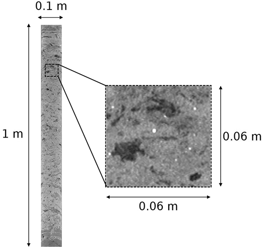
Ypresian clay, a marine clay regarded as a potential host formation for deep radioactive waste disposal in Belgium and the Netherlands, is selected as the natural material to investigate gas transport behaviour. A well-preserved, 1 m-long vertical core of Ypresian clay was retrieved from the DAPGEO-02 borehole at depth of 393 m (Vardon et al., 2022). The core was subsequently scanned using an X-ray medical scanner with a voxel resolution of 0.23 × 0.23 mm × 0.6 mm³ (Vardon et al., 2023). Figure 1 presents a vertical slice of the core, revealing a non-uniform distribution of material density and the absence of visible cracks.

The porosity distribution of the core is characterised by quantifying the average porosity of each voxel. The dry density is inferred from the Hounsfield unit (HU) value using the method proposed by Rogasik et al. (1999):

where HU represents the voxel intensity of the bulk material, which results from the combined contributions of the three phases: $HUs$⁠, $HUw$⁠, and $HUa$⁠, representing the voxel intensities of the solid, water, and air phases, respectively. By convention, $HUw$ is zero and $HUa$ is −1024. The volume fractions of the solid, water, and air phases are represented by $ϕs$⁠, $ϕw$⁠, and $ϕa$⁠, respectively, with: $ϕs=1−ϕ$⁠, $ϕw=ϕSw$⁠, and $ϕa=1−ϕs−ϕw$⁠, where $ϕ$ is the porosity and $Sw$ is the degree of saturation. The core is assumed to be fully saturated and therefore: $ϕa=0$⁠, $Sw=1$⁠. Rearranging Equation 1, the porosity per voxel can be obtained as follows:

where $HUs$ is assumed to be constant for any investigated soil. By considering Equation 1 for the entire core rather than a single voxel, $HUs$ can be expressed as follows:

where $HUcore$ is the average HU value of the core, $ϕscore$ is the volume fraction of the solid phase for the core, $ρbcore$ is the average bulk density of the core, $wcore$ is the average mass water content of the core, and $ρs$ is the density of the solid particles, which is assumed to be constant across the core.

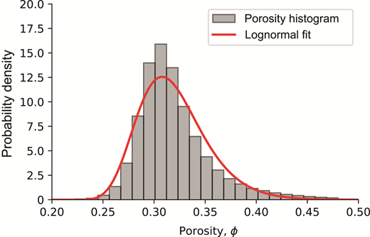
The solid particle density, bulk density, and mass water content of the core for Ypresian Clay were taken from literature (Piña Díaz, 2011): $ρs=2700$ kg m$−3$⁠, $ρbcore=2119$ kg m$−3$⁠, and $wcore=0.159$⁠. With these data, the porosity of each voxel in the core can be calculated using Equations 2 and 3. Consequently, the porosity distribution of the core is shown in Figure 2. The data were fitted using a log-normal distribution, resulting in a mean porosity of 0.322 and a standard deviation of 0.030. In addition, a trend in porosity was observed along the 1 m long core. The mean porosity of each XCT slice (with a thickness of 0.6 mm) decreases with depth from 0.34 to 0.31. As will be introduced later, the domain sizes used in the numerical analyses conducted in this study range from 10 mm to 80 mm, over which the effect of porosity trend is negligible. Consequently, a stationary random field with constant mean and standard deviation is assumed throughout the analysis.

The spatial correlation is characterised using a variogram analysis, which quantifies how the variance of properties between points changes as a function of distance, referred to as the lag distance. The semi-variance for each lag distance is calculated as follows:

where $Z(xi)$ and $Z(xi+rk)$ are the values of the variables at paired locations $xi$ and $xi+rk$ measured in a given direction. In this study, the variable Z represents the porosity, $rk$ is the k-th lag distance among a set of lag distances $r1,r2,...,rK$⁠, $N(rk)$ is the number of data pairs separated by $rk$⁠, and $γ(rk)$ represents the semi-variance of the data measured with the k-th lag distance. The variogram for a set of lag distances can be expressed as a vector:

The measured variogram, $γ(r)$⁠, typically increases with lag distance because points farther apart tend to exhibit lower correlation. The scale of fluctuation is related to the lag distance at which the variance reaches a stable value. Beyond this distance, the points are considered uncorrelated, indicating that spatial dependence no longer exists. The scale of fluctuation can be determined by fitting the measured variogram with various empirical models (Federico and Neuman, 1997).

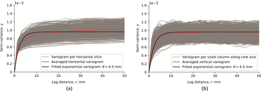
In this analysis, the empirical variograms are calculated both perpendicular to and parallel to the core axis using Equation 4, with the results presented in Figure 3. For the horizontal variograms (perpendicular to the core axis), individual variograms are calculated per horizontal slice (0.6 mm thickness), and indicated by grey lines. Within each slice, the sampling direction is arbitrary but confined to the plane of the slice. Sampling (lag) distances range from 0.5 mm to 50.0 mm, with constant increments of 0.5 mm. For each lag distance, 10,000 data pairs are randomly sampled. This sampling method aligns with the concept of a variogram family as proposed by Vogel (2001). By averaging the variograms from individual slices, an average horizontal variogram is obtained, as indicated by the red line in Figure 3(a). For the vertical variograms (parallel to the core axis), the variograms are calculated per voxel column in the direction of the core axis. As discussed above, the porosity trend with depth is removed, and the variograms are computed based solely on the variability due to local stochastic variation. Lag distances range from 0.6 mm to 50.4 mm with a constant increment of 0.6 mm. A total of 1,000 voxel columns are randomly sampled for the calculation. By averaging the variograms from individual voxel columns, an average vertical variogram is obtained (Figure 3(b)). Subsequently, the averaged horizontal and vertical variograms are fitted using the following empirical variogram model with an exponential correlation function (Lloret-Cabot et al., 2014):

where $σ$ is the standard deviation, and $θ$ is the scale of fluctuation.

An isotropic scale of fluctuation of 4.5 mm is considered to fit the variograms in both directions. Note that the voxel size of the CT scan (0.23 $×$ 0.23 $×$ 0.6 mm) is between 7.5 and 19.6 times smaller than the scale of fluctuation. This resolution is considered sufficiently high for the analysed material. Additionally, the nugget effect is not considered, because each voxel contains an averaged porosity value ‘upscaled’ from the clay particle and grain scale already, which means that there is no nugget effect possible in the classical definition of the nugget.

By adopting the above characterised parameters with a mean of 0.322, a standard deviation of 0.03, and a scale of fluctuation of 4.5 mm, random fields of porosity are generated using the randomisation method, which is a variation of the Fourier method (Heße et al., 2014), as implemented in GSTools (Müller et al., 2022). This method is based on discretising the spectral representation of a random field to simulate spatial variability (Shinozuka and Jan, 1972). It offers computational efficiency and flexibility, making it particularly suitable for generating large-scale random fields in geotechnical and geological applications.

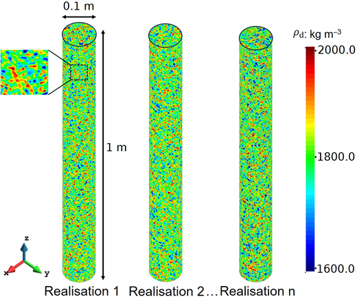
Figure 4 shows multiple realisations of random fields of dry density generated for a 3D model of the core sample depicted in Figure 1. The dry density was uniquely correlated to porosity using the relation $ρd=(1−ϕ)ρs$⁠, where $ρs$ is the density of the solid clay particles. The generated random fields demonstrates strong qualitative ability to reproduce the natural variability observed in the CT scan of the core (Figure 1), particularly the heterogeneous nature of dry density.

The finite element code LAGAMINE (Charlier, 1987; Collin et al., 2002) is used in this study. The theoretical framework considers a mixture composed of three species – mineral, water, and hydrogen – distributed in three phases – solid, liquid, and gas. Unless otherwise specified, the subscripts s, l, and g refer to the solid, liquid, and gas phase properties, while the superscripts w and $H2$ refer to the properties of water and hydrogen. In this formulation, the mineral species is assumed to coincide with the solid phase. The liquid phase contains both water and dissolved hydrogen, while the gas phase is treated as a perfect mixture of gas-phase hydrogen and water vapour. Hydro-mechanical coupled effects are neglected in this study, and the model is therefore reduced to a two-phase flow analysis.

Porosity is treated as a random variable, with its random field parameters characterised in the previous section. The random porosity field is translated into random fields of permeability, apparent diffusivity, retention properties, and relative permeability, using the formulations given in the following sections. These hydraulic properties may also exhibit variability due to factors other than porosity, such as mineralogy composition and pore size distribution. However, such sources of variability are not considered in this study, as they are difficult to quantify with the currently available data. It is recommended to characterise these sources of variability in future work when more data are available.

The compositional approach is adopted to establish the mass balance equations. It consists of balancing species rather than phases. Accordingly, the water and hydrogen mass balance equations are expressed as:

where $ρw$⁠, $ρgw$⁠, $ρgH2$⁠, and $ρlH2$ [kg m$−3$] are, respectively, the mass density of liquid water, water vapour, gas-phase hydrogen, and dissolved hydrogen, $Sw$ [-] is the degree of saturation, $ϕ$ [-] is the porosity, and $flw$⁠, $fgw$⁠, $fgH2$⁠, and $flH2$ [kg m$−2$ s$−1$] are, respectively, the mass fluxes of liquid water, water vapour, gas-phase hydrogen, and dissolved hydrogen.

The total gas pressure is equal to the sum of the partial pressures of gas-phase hydrogen and water vapour. The density of each species in the gas phase is assumed to be governed by the ideal gas law. It is given by:

where $MH2$ and $Mw$ [kg mol$−1$] are the molar mass of hydrogen and water species, $pgH2$ and $pgw$ are the partial pressure of hydrogen and water species in the gas phase, R is the universal gas constant (equal to 8.314 m³ Pa K$−1$ mol$−1$⁠), and T [K] is the system temperature.

The density of dissolved hydrogen, $ρlH2$ [kg m$−3$], is obtained with Henry’s law, assuming local equilibrium of the gas-phase hydrogen and the dissolved hydrogen:

where H is the dimensionless Henry solubility constant for the hydrogen dissolved in liquid water. The dissolved hydrogen is assumed to have a negligible effect on the density of the liquid phase. Consequently, the density of the liquid phase is assumed to be equal to the density of the liquid water, and it is calculated linearly by the liquid phase pressure:

where $pl$ is the liquid phase pressure, $1/χw$ [Pa$−1$] is the water compressibility, and $ρw,0$ is the liquid water density at the reference liquid pressure $pl,0$⁠. The partial pressure of the water vapour is governed by Kelvin’s equation as follows:

where $pg,0w$ [Pa] is the maximum vapour pressure, and $s=pg−pl$ [Pa] is the suction.

The mass fluxes in Equations 7 and 8 can be expanded for the water and gas species as follows:

where $fw$ and $fH2$ are the mass fluxes of the water and hydrogen species, $ql$ and $qg$ [m s$−1$] are the advective fluxes of the liquid and gas phases; $igw$⁠, $igH2$⁠, and $ilH2$ [kg m$−2$ s$−1$] are the diffusive mass fluxes of water vapour, gas-phase hydrogen, and dissolved hydrogen.

The advective fluxes are governed by the following two-phase extension of Darcy’s law:

where K [m²] is the intrinsic permeability of the porous medium, which is assumed to be isotropic, $μl$ and $μg$ [Pa s] are the dynamic viscosity of the liquid and gas phases, and $kr,l$ and $kr,g$ [-] are the dimensionless relative permeability of the liquid and gas phases. The intrinsic permeability is assumed to evolve with porosity according to the Kozeny-Carman expression (Chapuis and Aubertin, 2003):

where $K0$ [m²] is the reference intrinsic permeability at reference porosity $ϕ0$⁠. The model predicts an increase in fluid conductivity with increasing porosity.

The diffusive mass fluxes, $igw$⁠, $igH2$⁠, and $ilH2$ are governed by the Fick’s law for an unsaturated porous medium:

where $Sw$ [-] is the degree of saturation of the liquid phase, $Dgw$ and $DlH2$ [m s$−2$] are the diffusion coefficients of the water vapour and dissolved hydrogen, $τ$ [-] is a dimensionless coefficient that accounts for the influence of the tortuosity of the pore space. For a mixture of water vapour with any gas species, the diffusion coefficient is calculated as follows:

where $Dg,0w$ is the reference diffusion coefficient of the water vapour at $T0=273.15$ K and $pg,0=101.325$ kPa.

The water retention curve (WRC) of the porous medium is described by a modified van Genuchten model (Gallipoli et al., 2003), which introduces a dependence of the AEV on the void ratio. Accordingly, the degree of saturation is expressed as:

where e [-] is the void ratio, and A [Pa], $ψ$ [-], and n [-] are model parameters. The model describes how void ratio affects capillary retention and gas entry.

The relative permeability for gas and liquid phases used in Equations 16 and 17 is considered to be a function of the saturation degree. The liquid-phase relative permeability is determined using the Mualem-van Genuchten model (Mualem, 1976), while the gas-phase relative permeability is described by the cubic model:

where m is a parameter controlling the shape of the liquid relative permeability curve: $m=1−1/n$⁠.

2D plane-strain and 3D models with regular meshes are constructed for the gas injection tests. In the 2D models, square samples with side lengths, l, of 10, 20, 40, and 80 mm are analysed. For 3D models, cubic samples with side lengths of 10, 20, and 40 mm are considered. The 80 mm sample size is excluded in the 3D study due to the high computational cost. A square-shape element with a 2 mm side length is adopted for all 2D samples, while a cubic-shape element with the same side length is used for all 3D samples. To enable the analysis of the 3D 80 mm sample in future work, the implementation of an iterative solver (Saad, 2003) and parallel computing (Wang et al., 2015) may be beneficial, given the large number of degrees of freedom involved.

The initial gas pressure in the domain is set to 0.1 MPa, assuming that the samples are initially exposed to atmospheric pressure. The initial liquid pressure is set to 0.5 MPa, which is of the same order as typically applied in laboratory gas injection tests (e.g. in Arnedo et al., 2008; Gonzalez-Blanco et al., 2016; Harrington et al., 2019). Consequently, the soil is initially saturated with water, and the initial concentration of dissolved hydrogen is determined by Henry’s law (Equation 11). Gas injection is simulated by increasing the gas pressure at the bottom boundary (injection boundary) from 0.1 MPa to the target gas injection pressure, $pginj$⁠, and waiting for the system to reach a steady flow state. The injection boundary is set to be impermeable to water, while the lateral boundaries are set to be impermeable to both water and hydrogen. At the top boundary (back-pressure boundary), both gas and liquid pressures are fixed at their initial values, namely $pgback=$ 0.1 MPa and $plback=$ 0.5 MPa. Two gas injection pressures are considered, namely 5.0 MPa, which is referred to as the high gas injection pressure condition hereafter, and 2.0 MPa, referred to as the low gas injection pressure condition in this study. Consequently, four conditions are analysed, hereafter denoted HP2D, LP2D, HP3D, and LP3D, where ‘HP’ and ‘LP’ represent high and low gas injection pressure conditions, respectively, and ‘2D’ and ‘3D’ refer to two-dimensional and three-dimensional analyses, respectively.

Table 1 summarises the analyses conducted, including deterministic analyses with homogeneous porosity and stochastic analyses with randomly assigned porosity. In the deterministic analysis, simulations are performed for four sample sizes with mean porosity (0.322) under the HP2D condition to assess the impact of sample size on the deterministic results. Then, the effects of porosity are evaluated by assigning different porosities to the 20 mm sample under the HP2D condition. Three distinct porosity levels were considered: the lower bound (0.25), mean value (0.322), and upper bound (0.4). The lower and upper bounds correspond to the 1st and 99th percentile of the measured porosity distribution (Figure 2) for the Ypresian clay. In the stochastic analysis, the same random field parameters for porosity are adopted for all conditions. For each sample size, 2000 realisations are performed, except for the 40 mm sample under 3D conditions (HP3D and LP3D), where 1000 realisations are conducted for saving computational cost. All statistical results (e.g. the coefficient of variation) stabilise within the number of realisations performed.

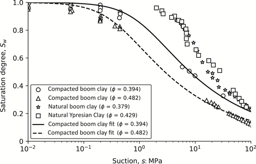
The hydraulic properties of the soil and the fluid properties adopted in this study are presented in Table 2. The reference porosity is set to be the mean porosity (0.322) as characterised in the previous section. The reference intrinsic permeability corresponding to the reference porosity is adopted from Piña Díaz (2011) for Ypresian Clay with a similar porosity. The water retention properties of Ypresian Clay at different void ratios are unavailable for calibrating Equation (22). Instead, the calibration was performed using compacted Boom Clay data for two reasons. First, Ypresian Clay and Boom Clay have similar clay content and mineralogical composition (Piña Díaz, 2011; Zeelmaekers et al., 2015). Second, their water retention curves are similar, as shown in Figure 5. Based on this, the tortuosity of Boom Clay (Jacops et al., 2013) was adopted. The properties of water and hydrogen are presented in Table 2.

This section presents the results of deterministic analysis conducted under the assumption of a homogeneous material. The purpose of the deterministic analysis is to evaluate the effects of sample size and porosity on the sample average saturation degree, time to reach steady flow state, and the gas transport mechanism. First, the effects of sample size are examined; second, the influences of porosity are evaluated. All deterministic analyses are performed under 2D conditions, as the results are identical for 2D and 3D analyses when homogeneous material properties are considered.

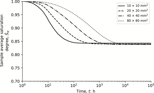
Taking conditions of high gas injection pressure (HP2D) as an example, Figure 6 illustrates how sample size influences the sample average saturation degree, $S¯w$⁠, referred to as the sample saturation degree hereafter for simplicity. The sample saturation degree is defined as the ratio of the pore volume filled with liquid to the total void volume of the soil sample. This variable is measurable in laboratory gas injection tests and directly influences the gas permeability of the sample. Figure 6 shows that the sample saturation degrees at the steady state are practically the same across all sample sizes, since the same gas injection pressures are applied consistently to samples of varying sizes, resulting in similar suction levels across all samples. In addition, Figure 6 shows that larger samples take longer to reach a steady state. This is because larger samples have greater pore volume, increasing gas storage capacity for the same sample saturation degree at steady state. Consequently, more time is required for the gas to fill the pores before achieving a steady flow state.

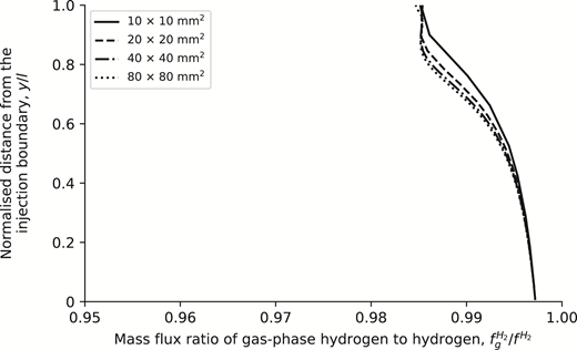
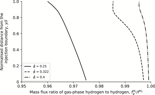
Figure 7 shows the profiles of the mass flux ratio of gas-phase hydrogen to hydrogen across the sample, from the gas injection boundary to the back pressure boundary, for different sample sizes. The mass flux of hydrogen includes both gas-phase hydrogen and dissolved hydrogen. The results show that the proportion of gas-phase hydrogen decreases from the injection boundary to the back pressure boundary, since the gas pressure and liquid pressure are fixed at 0.1 and 0.5 MPa, respectively, at the back-pressure boundary, leading to a high saturation degree near the boundary. Nonetheless, the proportion of gas-phase hydrogen is higher than 95% across all samples. This suggests that at steady state, the gas migration behaviour is primarily governed by the advection and diffusion of the gas-phase hydrogen, which is strongly influenced by the gas saturation degree and gas relative permeability. In contrast, the dissolved gas outflow is negligible. The above findings are also valid for the conditions of low gas injection pressure (LP2D).

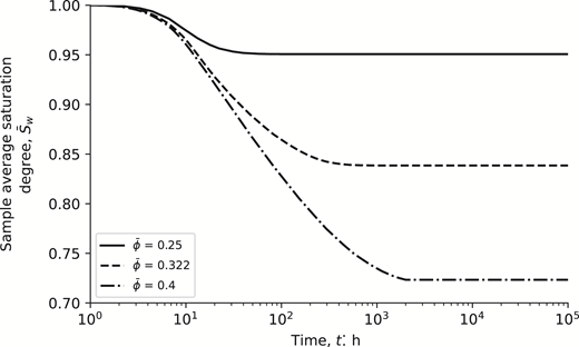
To evaluate the effects of porosity, Figure 8 presents the evolution of the sample saturation degree for the 20 mm sample with the different porosities: 0.25, 0.322, and 0.4, using condition HP2D as an example. The results show that the sample saturation degree at steady state decreases with increasing porosity, and the lower and upper limits are 0.72 and 0.95. In addition, samples with larger porosity take longer to reach steady-state saturation levels. This is primarily due to increased porosity resulting in larger pore volumes and a lower AEV, as described in Equation 22. A lower AEV causes greater desaturation under the same gas injection pressure. These factors contribute to a higher gas storage capacity, thereby extending the time required to reach a steady-state saturation level, as mentioned before. Conversely, increased porosity also raises water conductivity, which reduces the time needed for the gas-phase hydrogen to displace water from the pores. Overall, the results suggest that the dominant mechanism governing the behaviours is the increased gas storage capacity.

Figure 9 illustrates that the ratio of gas-phase hydrogen to hydrogen decreases with decreasing porosity. This occurs because lower porosity results in a higher saturation degree, which reduces the gas relative permeability and increases the apparent gas diffusivity in water, leading to a lower proportion of gas-phase hydrogen. Despite this, gas-phase hydrogen remains the dominant transport mechanism (>95%) compared to dissolved hydrogen across all considered porosities. The above findings are also valid for condition LP2D.

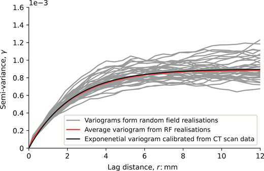
Before proceeding with the stochastic analysis, a quantitative verification of the random field generator was performed. For this purpose, variograms were computed from 200 realisations of random fields generated for the 20 mm sample, following the same procedure previously applied to the CT scan data of the Ypresian clay core. The resulting variograms are shown as grey curves in Figure 10, along with the average variogram (in red) and the exponential variogram fitted to the CT scan data of the clay core (in black). As expected, the average variogram from the random field realisations closely matches the exponential model calibrated from the CT scan, confirming the validity of the generator.

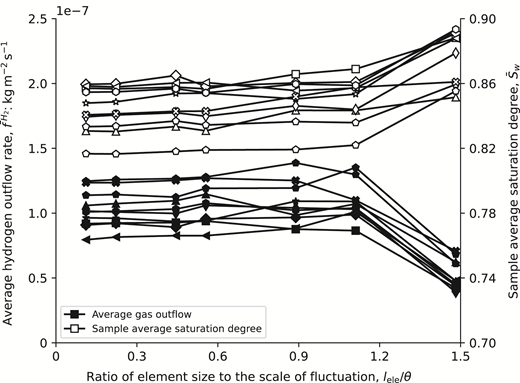
Since random porosity is considered in the analysis, the mesh size may influence the accuracy of capturing the heterogeneous distribution of porosity, which in turn can affect the modelling results. To evaluate the effects of the mesh, seven elements sizes are considered, leading to a ratio of element size to the scale of fluctuation (⁠$lele/θ$⁠) ranging from 0.1 to 1.5. Figure 11 shows the influences of mesh size on the average hydrogen outflow rate and the sample saturation degree at the steady state, taking the 20 mm sample under HP2D condition as an example. The average hydrogen outflow rate, $f¯H2$ [kg m$−2$ s$−1$], is defined as the total mass rate of hydrogen [kg s$−1$] flowing out through the outflow boundary divided by the cross-sectional area of the boundary. Ten random field realisations are considered, which are represented by different marker shapes. The white markers correspond to the results of sample saturation degree, while the black markers represent the results of average hydrogen outflow rate. The results demonstrate that both sample saturation degree and average hydrogen outflow rate show practically no mesh dependency for $lele/θ<0.5$⁠. Similar mesh sensitive analysis were performed for other sample sizes yielding similar results. This observation is consistent with Huang and Griffiths (2015), who recommend that for a quadrilateral element with four integration points (two in each Cartesian direction), the ratio of element size to the scale of fluctuation should be less than 0.5 to accurately capture the random variable. Based on this, an element size of 2 mm (⁠$lele/θ=0.44$⁠) is adopted for all analyses in this study. This element size is assumed to be sufficiently small to accurately represent the considered porosity random fields under both 2D and 3D conditions.

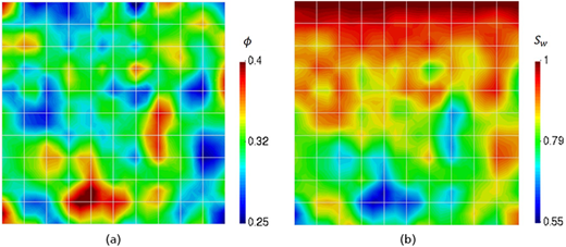
With the adopted element size, Figure 12 shows the 2D mesh for the 20 mm sample. For visualising the generated random field, Figure 12(a) shows the distribution of random porosity for a single realisation. As mentioned before, the porosity ranges from ≈0.25 to 0.4, representing the 1st and 99th percentile of the measured porosity distribution (Figure 2). It is also demonstrated that the porosity is correlated within the distance of the scale of fluctuation (4.5 mm) in certain regions. Figure 12(b) shows the distribution of saturation degree at a steady flow state under condition HP2D. The results show that the desaturation is more significant in the area with larger porosity, where the gas preferentially flows, as shown in Figure 18(a). However, the region near the outflow boundary remains nearly fully saturated because the gas pressure and liquid pressure are fixed at 0.1 MPa and 0.5 MPa, respectively, at the boundary, leading to low suction near the boundary.

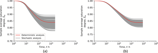
To demonstrate the effects of heterogeneity on the sample saturation degree and the time to reach steady flow state, Figure 13 shows the evolution of the sample saturation degree for 20 and 40 mm sample sizes under condition HP2D. The red lines represent the deterministic results and the grey lines represent the stochastic results based on 200 realisations using the same random field input parameters. For the sample saturation degree, the plots show that the variation decreases as the sample size increases from 20 to 40 mm. This is because there are more averaging effects in larger sample sizes. For the time to reach the steady state, the result shows that it increases significantly from the 20 mm sample to the 40 mm sample for both deterministic and stochastic analyses. Moreover, for each sample size, the time to reach the steady state increases as the steady-state sample saturation degree decreases. These observations are consistent with the previous explanation that a higher gas storage capacity – provided by a larger volume and lower saturation degree – leads to longer duration to achieve the steady flow state.

In addition to the sample saturation degree, the equivalent gas permeability, $k¯g$ [m²], is also a key variable measured in the laboratory for evaluating the conductivity of the sample to gas. In this study, the equivalent gas permeability is calculated from the average hydrogen outflow rate, $f¯H2$⁠. Given that the transport of hydrogen is dominated by the gas-phase hydrogen (Figures 7 and 9) and is assumed to be governed by advection, the equivalent gas permeability is defined as follows:

where $f¯H2$ [kg m$−2$ s$−1$] is the average hydrogen outflow rate, l [m] is the side length of the sample, $ρgSTP$ [kg m$−3$] is the gas density of hydrogen under standard temperature and pressure (STP) conditions, equal to 0.089 kg m$−3$⁠, and $pginj$ and $pgback$ [Pa] are the gas injection pressure and back pressure, respectively.

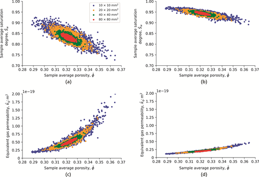
Figure 14 shows correlations of the sample average porosity with both the sample saturation degree and equivalent gas permeability at the steady state for different sample sizes. Figures 14(a) and 14(c) correspond to the condition of high gas injection pressure and Figures 14(b) and 14(d) are for the condition of low gas injection pressure. A total of 2000 realisations are considered for each sample size. The sample average porosity is defined as the ratio of the total void volume within the sample to the total volume of the sample and is referred to simply as ‘sample porosity’ hereafter for brevity. The results show that variations in both the sample saturation degree and equivalent gas permeability decrease as the sample size increases. Taking the 20 mm sample as an example, the lower and upper bounds of the sample saturation degree in the stochastic analysis fall within the bounds observed in the deterministic analysis, as shown in Figure 8.

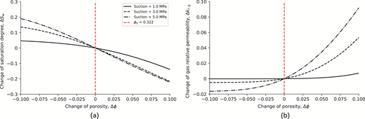
Comparing the conditions of high (HP2D) and low gas injection pressure (LP2D), the sample saturation degree is significantly higher under low gas injection pressure, and the equivalent gas permeability at steady state is much lower. This is because the suction is lower under low gas injection pressure, leading to a higher saturation degree and lower gas relative permeability. In addition, both sample saturation degree and equivalent gas permeability show less variation in the condition of low gas injection pressure, as indicated by the narrower bandwidth observed in Figures 14(b) and 14(d) compared to Figures 14(a) and 14(c). This can be explained by Figure 15, which shows the effects of porosity variations on changes in saturation degree (Figure 15(a)) and gas relative permeability (Figure 15(b)) for three different suction levels. The curves are plotted according to the water retention (Equation 22) and gas relative permeability (Equation 24) models adopted in this study. The red vertical dashed line indicates the starting point of the variation, corresponding to the mean porosity $ϕ¯$ used in the deterministic analysis. Figure 15 shows that an increase in porosity leads to a decrease in saturation degree and an increase in gas relative permeability at a given suction level. The plot also shows that the variation of both saturation degree and gas relative permeability due to porosity changes is weaker at low suction levels than at high suction levels. Consequently, the results show less variability in the condition of low gas injection pressure.

Since the effects of gas-induced cracking (Guo and Fall, 2019; Liaudat et al., 2023) are not considered, the model is not able to capture the effects of cracking on the hydraulic properties of the material, such as the enhancement of the permeability and the reduction of the AEV. Consequently, the simulation predicts varying degrees of desaturation during gas injection (Figures 14(a) and 14(b)), which is inconsistent with experimental observations showing that the soil sample remains almost fully saturated after a gas injection test (e.g. Harrington and Horseman, 1999). This discrepancy arises because preferential gas flow occurs through the cracking zones in the experiments, without de-saturating the bulk clay materials.

The effect of gas-induced cracking can be captured by explicitly modelling the propagation of gas fractures using interface elements (Liaudat et al., 2023) or phase field methods (Guo and Fall, 2019). Alternatively, it can be captured implicitly by coupling hydraulic properties with ‘embedded fractures’, which are driven by deformation (e.g. Damians et al., 2022; Rodriguez-Dono et al., 2023). The variability of the modelling results may differ if the effects of gas-induced cracking are taken into account. Nonetheless, as an initial step, the results of this study provide preliminary insights into the variability of the overall responses in gas injection tests.

This section presents the results of stochastic analyses under 3D conditions, including conditions HP3D and LP3D considering sample sizes of 10, 20, and 40 mm, as listed in Table 1. In addition, the statistical results under 3D conditions are compared with those under 2D conditions. The comparison first focuses on the mean of the 2D and 3D statistical results, followed by comparing the variability of the results between 3D and 2D conditions.

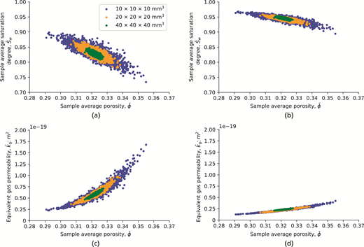
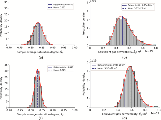
Under 3D conditions (HP3D and LP3D), the correlation of the sample porosity with the sample saturation degree and the equivalent gas permeability is presented in Figure 16. The results exhibit a similar trend to those observed under 2D conditions (Figure 14). Taking the 20 mm sample as an example, Figure 17 compares the mean of the statistical results between 2D and 3D conditions, along with a comparison with the deterministic result. The figure shows the histogram of the sample saturation degree (Figures 17(a) and 17(c)) and the equivalent gas permeability (Figures 17(b) and 17(d)) for both 3D and 2D conditions. The histograms are fitted with log-normal distributions indicated by the red lines. In addition, the deterministic result and mean of the stochastic analysis are included in the figures and represented by the blue solid line and blue dashed line, respectively. The results indicate that the mean of the sample saturation degree obtained from stochastic analysis is lower than the deterministic result, both for 2D and 3D conditions. This can be explained by the non-linear relationship between porosity and saturation degree depicted in Figure 15(a). The figure shows that a decrease in saturation degree is greater than the corresponding increase for the same amount of porosity variation. This suggests that, in heterogeneous porous media, larger porosity regions have a greater influence on saturation and drain more easily during gas injection, leading to localised desaturation. In addition, the mean saturation degree is approximately the same between the 2D and 3D conditions.

For the equivalent gas permeability, the mean of the stochastic results is higher than the deterministic result (Figures 17(b) and 17(d)) due to the non-linear influence of porosity changes on variations in the relative gas permeability. As shown in Figure 15(b), the increase in gas relative permeability is much greater than the corresponding decrease for the same amount of porosity variation. This indicates that gas relative permeability is more sensitive to regions with higher porosity, leading to an overall increase in the mean equivalent gas permeability in stochastic analyses. However, this difference between the stochastic mean and the deterministic result is pronounced only in 3D conditions (Figure 17(d)), whereas in 2D conditions, it becomes nearly negligible (Figure 17(b)). Therefore, the deterministic equivalent gas permeability can be used to estimate the mean equivalent gas permeability of a stochastic analysis under 2D conditions, while under 3D conditions the deterministic result underestimates the mean equivalent gas permeability. This observation highlights the importance of considering 3D effects when modelling gas flow in heterogeneous media. The above findings are also valid for other sample sizes.

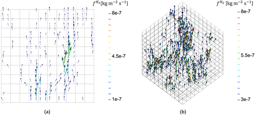
The above observation regarding the gas permeability can be explained by comparing the gas flow patterns under 2D and 3D conditions, as depicted in Figure 18 for the 20 mm sample. Figure 18(a) shows the pattern of hydrogen flux in steady state for the 2D condition, with the corresponding patterns of porosity and saturation degree shown in Figures 12(a) and 12(b), respectively. Figure 18(b) shows the hydrogen flux pattern for the 3D condition, using the same heterogeneity seed as in the 2D condition, resulting in a similar saturation degree to that of the 2D condition. By comparing Figures 18(a) and 12(b), it is shown that gas preferentially flows through areas with larger porosity and lower saturation degree. However, this preferential flow is obstructed when the gas encounters regions with smaller porosity and higher saturation degree. In comparison, under 3D conditions, there are more opportunities for connecting areas with high porosity (Figures 18(a) and 18(b)), confirming preferential gas flow pathways through the sample, leading to higher sample gas permeability. Alternatively, this observation could be interpreted by appealing to the percolation theory, which predicts a lower percolation porosity threshold in 3D domains compared to 2D (e.g. Wang et al., 2022). This observation indicates that the equivalent gas permeability is not only controlled by the average sample saturation degree, but is also influenced by the spatial distribution of saturation degree within the sample. The above findings are consistent with previous studies on stochastic analysis of hydraulic conductivity (e.g. Griffiths and Fenton, 1997) that the mean increases in 3D conditions as compared to 2D conditions.

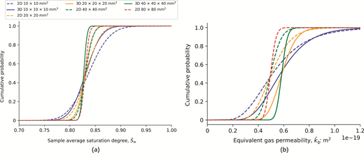
To compare the distributions of the statistical results between 2D and 3D conditions for various sample sizes, Figure 19 shows the cumulative distributions of sample saturation degree (Figure 19(a)) and equivalent gas permeability (Figure 19(b)) for 10, 20, and 40 mm samples under conditions HP2D and HP3D. Solid lines represent the 3D condition, while dashed lines represent the 2D condition. The cumulative distributions are derived based on the fitted log-normal distribution depicted in Figure 17, taking the 20 mm sample as an example. Figure 19(b) shows that, under high gas injection pressure (conditions HP2D and HP3D), the cumulative distributions in 3D shift to the right relative to the 2D condition, suggesting that the equivalent gas permeability increases from the 2D to the 3D condition. This observation aligns with the above explanation that the high gas relative permeability regions are more likely to be connected under 3D conditions than under 2D conditions (Figure 18). The 3D effects described above for the high gas injection pressure condition have also been observed under the low injection pressure condition.

The following discussion considers the variability of the statistical results between 3D and 2D conditions. Figure 19(a) shows that, under high gas injection pressure (conditions HP2D and HP3D), the cumulative curves of the sample saturation degree for the 3D condition are narrower than for the 2D condition. This is because the averaging effects are more significant in the 3D condition, leading to less variation. Similarly, Figure 19(b) shows that the cumulative curves of the equivalent gas permeability in the 3D condition are also narrower compared to those in the 2D condition, indicating reduced variation of equivalent gas permeability due to enhanced averaging out effects under 3D conditions.

The above findings align with the observations from Figures 14 and 16, where the scatters representing the sample saturation degree and the equivalent gas permeability are more concentrated in 3D conditions than in 2D conditions. In addition, the ranges of the scatters between the upper and lower bounds are narrower for 3D conditions compared to 2D conditions. The effects of reduced variability in 3D conditions, as described above, are observed under both high and low gas injection pressure conditions. The above findings are consistent with previous studies on stochastic analysis of hydraulic conductivity (e.g. Griffiths and Fenton, 1997) that the variability decreases from 2D to 3D conditions.

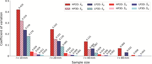
Figure 20 presents the coefficients of variation from the stochastic analysis for the equivalent gas permeability and sample saturation degree at steady state under both high and low gas injection pressures conditions for different sample sizes. Both 3D and 2D conditions are considered except for the 80 mm sample size in the 3D condition. Figure 20 shows that the coefficient of variation for the equivalent gas permeability is much higher than that for the sample saturation degree. This indicates that the variation in the equivalent gas permeability is considerably greater than that in the sample saturation degree. For the equivalent gas permeability, the coefficient of variation under low gas injection pressure is significantly lower than under high gas injection pressure; that is approximately half as large. Besides, the coefficient of variation of the equivalent gas permeability under 3D conditions is much lower than under 2D conditions, with this difference being more pronounced for larger sample sizes: under both high and low gas injection pressure conditions, the coefficient of variation of the equivalent gas permeability in 3D is ≈75%, 60%, and 45% of that in 2D for the respective sample sizes. Notably, when the sample size increases to 40 mm, the coefficient of variation for the equivalent gas permeability in 3D analysis becomes lower than that of the 80 mm sample in 2D analysis. This highlights the influence of 3D effects in reducing variability due to greater spatial averaging.

The coefficients of variation presented in Figure 20 for 3D samples provide an estimation of the variability that can be expected in experimental studies on Ypresian clay as a function of sample size. The minimum number of tests required to evaluate the mean response with a 95% confidence can be calculated using the following formulation Montgomery and Runger (2010), provided that the variables follow a log-normal distribution:

where E denotes the relative error margin and $Eμ$ represents the absolute error margin. The term COV refers to the coefficient of variation of the analysed result, such as the sample degree of saturation or gas permeability.

According to Equation 26 and the coefficients of variation provided in Figure 20, the minimum number of tests necessary to evaluate the mean gas permeability with relative error margins of 5% and 10% is provided in Table 3. The calculations are based on the coefficients of variation obtained from 3D simulations, except for the 80 mm³ sample, where the results are derived from 2D simulations. It is noteworthy that the number of required tests derived from the 80 mm² sample size in 2D conditions is more than for the 40 mm³ sample size in 3D conditions. This highlights again the importance of considering 3D effects, which lead to enhanced averaging and reduced variability. For the sample average saturation degree, since the coefficients of variation are small (Figure 20), the minimum number of tests required to achieve relative error margins of 10% and 5% is one for all sample sizes under both conditions of high and low gas injection pressures.

In addition to the required number of tests, Table 3 also lists the average duration [d] required to reach a steady state, as obtained from the stochastic analysis for each sample size. The steady state is assumed to be reached when the difference between the current and the final sample saturation degree is less than 0.1%.

According to Table 3, in order to evaluate the mean of the equivalent gas permeability with a desired level of accuracy, the required number of tests is significantly affected by the sample size. Specifically, the required number decreases with increasing sample size, although this comes at the cost of longer test duration. Therefore, selecting the appropriate sample size requires balancing the number of required tests and the test duration based on the required gas injection pressure and the desired accuracy of the results.

It should be noted that the results presented in Table 3 are qualitative, and incorporating mechanical coupling that accounts for gas-induced cracking effects is required in future work to obtain more quantitative results.

A stochastic analysis of two-phase flow in clays was conducted, incorporating spatially correlated random fields of porosity. The impact of spatially correlated heterogeneity on results was evaluated for different sample sizes and gas injection pressures, as was the impact of considering spatial correlation in 2D and 3D simulations. The main findings of this study are provided as follows:

• The variability of the results, including the average sample saturation and the equivalent gas permeability at steady state conditions, decreases with increasing sample size due to the greater averaging effects in larger samples. For each sample size, the variability of the equivalent gas permeability is significantly higher than that of the sample saturation degree.

• The variation in results is shown to be higher under high gas injection pressure compared to low gas injection pressure. This is due to the fact that higher suction levels lead to greater variability in both the saturation degree and the gas relative permeability. This, in turn, increases the overall variability in the gas flow behaviour.

• The variability of the results under 3D conditions is significantly lower than under 2D conditions, with this difference becoming more pronounced as the sample size increases. Under both high and low gas injection pressure conditions, the coefficient of variation of the equivalent gas permeability in 3D is ≈75%, 60%, and 45% of that in 2D for the respective sample sizes. This observation underscores the impact of 3D effects in reducing variability through enhanced spatial averaging.

• Under 2D conditions, the deterministic equivalent gas permeability is comparable to the mean equivalent gas permeability in stochastic analysis. However, under 3D conditions, the deterministic value underestimates the mean due to the development of preferential gas flow paths, which allows for more efficient gas migration compared to 2D conditions.

• The mean of the sample saturation degree in the stochastic analysis is lower than the deterministic result. This occurs because, in heterogeneous porous media, larger porosity regions have a greater influence on saturation and drain more easily during gas injection, leading to localised desaturation.

• Sample size is a critical factor in experimental design, as it influences the number of tests required to achieve results within a desired level of accuracy. Selecting an appropriate sample size requires balancing the number of tests and the test duration based on the applied gas injection pressure and the desired accuracy of the results.

Hydro-mechanical coupled effects were intentionally excluded in this study to isolate and evaluate the impact of heterogeneity on gas transport processes. The results provide a preliminary basis for future comparisons with studies that incorporate hydro-mechanical coupled effects. To obtain quantitative recommendations for experimental design, further developments are required to incorporate this mechanical coupling, including the potential development of discrete gas-induced paths, which have been observed in laboratory studies. Furthermore, additional experimental data is needed to describe the dependency of hydro-mechanical properties on porosity.

This study was conducted as part of the European Joint Programme on Radioactive Waste Management, which is funded by the European Union’s Horizon 2020 research and innovation programme under Grant Agreement Nos. 847593 (EURAD-GAS) and 101166718 (EURAD-2-HERMES). The first author acknowledges the support of the China Scholarship Council (CSC) and the Geo-Engineering Section at Delft University of Technology, the Netherlands.