
A model for predicting the settlement trajectory in saturated fluid fine tailings deposits is described. The model uses a population growth function and leverages established theories in soil mechanics, clay–water surface interactions and biogeochemistry to derive compressibility and permeability functions for predicting the settlement behaviour of fine tailings in deep deposits, typical of end pit lakes. The method is particularly useful for tailings treated with flocculants and/or coagulants with continuously changing compressibility and permeability parameters during deposition. For oil sands or mineral sands fluid tailings treated with or without high doses of a coagulant and/or a flocculant, the consolidation parameters determined from the model are comparable with those measured using standardised large-strain consolidation methods, and the predicted settlement using a modified Gibson’s finite-strain equation closely describes the measured settlement and void ratio profiles in geocolumns.
Notation
- A
Hamaker constant (zJ)
- Ab
unit basal area
- az
particle acceleration
- Ce
shape parameter or characteristic time factor
- c
electronic charge
- D
average particle diameter (m)
- ∂e/∂t
deformation rate
- de/dσ′
compressibility
- e
void ratio
- e0
initial void ratio
- e∞
void ratio at infinite time
attractive force
normal force exerted by the liquid on the platelet
repulsive force
sum of the forces on the clay platelet in the z direction
- f(x)
specific growth rate that depends on the concentration (x)
- GA
energy of attraction
- GB
Born energy
- GR
energy of repulsion
- GT
total interaction potential energy
- Gvdw
van der Waals energy
- g
acceleration due to gravity
- g(t)
lag function
- h
separation distance between particles
- hs
height of compressible soil skeleton
- K
reciprocal of the bound fluid thickness approximately at the centre of gravity of the electrical double layer
- k(e)
hydraulic conductivity (m/s)
- L
characteristic grain size (m)
- n
log-logistic function rate
- n0
ions per unit volume (ions/m3)
- R
average particle radius (m)
- S
per cent saturation
- SA
specific surface area of the particle
- T
absolute temperature
- t
time (s)
- tp
particle thickness
- t50
time at 50% deformation (s)
- u
hydrostatic stress (kPa)
- Ve0
equivalent mono dispersed spherical size of aggregate at the initial void ratio
- Ve∞
equivalent mono dispersed spherical size of the dehydrated aggregate
- Vp
particle volume
- Vv
volume of water around the particle and the non-interacting void spaces
- v
valency of ions
- x
concentration
- x0
initial concentration
- x∞
maximum concentration at infinite time
- y, z
dimensionless potential functions
- z
solid volume (m3)
- β
material constant that is directly related to the compressibility of the coagulant and flocculant
- Γ
surface charge density (C/m2)
- ε0
permittivity of vacuum
- εr
permittivity of the fluid
- κ
Boltzmann constant (J/K)
- μ
viscosity of water (Pa s)
- ξ
distance function
- ρL
density of the compressible component in the liquid phase
- ρp
particle density
- ρs
solids density (kg/m3) or solid specific gravity
- ρw
water density (kg/m3) or water specific gravity
- σ
total vertical stress (kPa)
- σ′
effective stress (kPa)
average effective stress (kPa)
- σA
stress resulting from attractive force per unit basal area
- σR
stress resulting from the repulsive force per unit basal area
- ψ
electric potential (mV)
- ψ0
electric potential at the particle surface (mV)
- ∇
gradient operator (i(∂/∂x) + j(∂/∂y) + k(∂/∂z))
Introduction
Bitumen extraction from surface-mined oil sands in Northern Alberta, Canada, generates approximately 1.2 barrels of fluid tailings for every barrel of bitumen produced. As of 2020, over 1400 million m3 of fluid fine tailings is stored behind several out-of-pit dyke structures (or tailings ponds) in the region (AER, 2021). During the life of a mine, the tailings pond doubles as a temporary storage facility for fluid tailings and a recycle water basin for bitumen extraction. After the end of mine life, fluid tailings footprints are expected to be reclaimed into terrestrial or aquatic landforms within the boreal forest ecosystem. The main reclamation challenge of fluid fine tailings is the centuries-long settlement and consolidation timelines stemming from the presence of very fine clay minerals (ARC, 1995) in the tailings slurry and the sheer volume of the fluid fine tailings. The reclamation challenge is a major hindrance to the sustainability of oil sands mining.
Prediction of the settlement trajectory during and after deposition of fine tailings in-pit or within a dyke structure with minimal uncertainty is also an ongoing challenge. During the deposition period, which may vary from months to decades, predicting the settlement trajectory is important for planning the required containment through the life of the asset. If the fine tailings deposit end state is a pit lake, settlement of the fine tailings sediment may continue for decades or centuries, during which the expressed water flux and ions into the water column may impact the aquatic ecosystem in the pit lake. The prediction uncertainty is exacerbated by the addition of high dosages of coagulants and/or flocculants to accelerate the initial settlement of the deposit.
The most common settlement prediction approach is to measure the compressibility and the hydraulic conductivity of a sample of the fine tailings using a large-strain consolidation (LSC) apparatus (Pollock, 1988), carrying out a seepage-induced consolidation (SIC) test (Znidarcic et al., 2011), using a geotechnical centrifuge or performing other modified oedometer methods. Consolidation tests can take weeks to months depending on the fine tailings slurry composition and the number of loading steps. The consolidation parameters are material properties input into a finite-strain equation to obtain the deposit settlement trajectory and excess pore pressure dissipation after placement (Gibson et al., 1967). Jeeravipoolvarn et al. (2008) modified Gibson’s finite-strain equation to model the settlement and consolidation behaviour of different oil sands fluid fine tailings deposits based on the measured consolidation and hydraulic conductivity properties of the fluid fine tailings. They reported very good agreement with experimental standpipes (Jeeravipoolvarn et al., 2008). The numerical model by Jeeravipoolvarn et al. (2009), packaged as FSCA, includes an interaction coefficient for coupling sedimentation to Gibson’s equation and is used as a comparative baseline to the log-logistic (LL) model developed in this study. The deformation rate obtained from Gibson et al.’s finite-strain equation is highly dependent on the compressibility and permeability functions, which often do not adequately describe the sedimentation portion of the settlement profile. This limitation is most acute in treated tailings deposits where the initial settlement rate is critical to pond elevation management and where the fabric of the clay aggregates in the deposit is continuously changed by chemicals (coagulants and/or flocculants) used to modify the mineral surface properties and accelerate the initial settlement phase. More recently, Zheng and Beier (2021) introduced a coupled model to simulate the settlement in oil sands fluid tailings deep deposit. Their model couples an unsaturated flow model with Gibson’s equation to simulate settlement (and water flux) in a fluid tailings deep deposit with a reclamation cover.
The works described earlier require significant sampling and consolidation testing of actual deposit samples as inputs into the settlement models. The method described in this paper uses a population growth function to describe the settlement trajectory derived from the Kozeny–Carman hydraulic conductivity function and interaction energies at the clay–water interface without the need for LSC measurements. The method is particularly suited for a tailings treatment facility with rapidly changing process variables that may have a significant impact on the sedimentation and primary and secondary consolidation phases of the settlement. While the theories behind the settlement model described in this paper are not particularly novel, the goal is to leverage established theories in soil mechanics, colloidal science and biogeochemistry to describe settlement as a response to changes occurring at the mineral–water interface.
Background
Settlement function
The equations developed by Gibson et al. (1967, 1981) to describe saturated clay deposits undergoing large deformations have been the workhorse for predicting the deformation rate (∂e/∂t) of fine tailings in deep deposits:
The equation is formulated in the Lagrangian coordinate where the boundary conditions at t = 0 are always the reference point. Here, e is the void ratio; ρ s and ρ w are the densities of the solid fabric and water, respectively; and z is the volume of the solid fabric. The equation assumes that the solid fabric is incompressible and the hydraulic conductivity, k(e), depends only on the void ratio. In deposits with drainage, the soil fabric (or soil skeleton comprising the solid fabric and the saturated pore space) is compressible with volumetric changes following de/dσ′. Note that Equation 1 is sometimes formulated in the form of de/dh s rather than de/dz, where h s is the compressible soil skeleton. Both the hydraulic conductivity and the compressibility (de/dσ′) of the deposit are typically measured on a subsample of the deposit. This requirement for sample measurement is often onerous in large inhomogeneous deposits where several measurements may be required to represent the deposit adequately. Besides, the common measurement methods (LSC, SIC) require modifications to incorporate sedimentation at low effective stresses and creep effects (secondary consolidation), which may be significant in deposits with residual hydrocarbons or treated with polymeric flocculants. An attempt is made in this paper to describe the compressibility and hydraulic conductivity as continuous functions from very high void ratios to the equilibrium void ratio in a deposit regardless of the settlement path taken to get to equilibrium (includes sedimentation, consolidation and creep), using a population growth model to describe the deformation rate ∂e/∂t.
The use of population growth models to describe system evolution over time is ubiquitous in biological and chemical processes as well as in economics. In its simplest form, the evolution of a population in an environment from time t = 0 to infinity is described by the first-order differential equation
f(x) is the specific growth rate that depends on the concentration (x). In this case, f(x) is a continuous function for all concentrations from an initial concentration x 0 to x ∞ (maximum concentration at infinite time), f(x 0) > 0 and f(x ∞) = 0. The specific growth rate function is highly dependent on the limiting growth parameter in the environment. Logistic growth starts with a period of exponential increase followed by a decay in the growth rate as the concentration approaches the carrying capacity. In an environment where the growth includes an induction time, typical of adaptation to a new environment, Baranyi et al. (1993) introduced a lag function (g(t)) into the differential equation:
A solution to this equation is a log-logistic function (LLF) first proposed by Barcroft and Hill (1910) and could be written as
Here, n is the logistic growth rate and t 50 is the time at 50% of the concentration between x 0 and x ∞. This LLF is shown here to describe adequately the settlement trajectory in a fine tailings deposit where the total stress and the solids volume are conserved. The method allows treatment of the sedimentation (includes the induction and the exponential growth (or particle aggregation) phases), primary consolidation and creep phases as a continuous function dependent solely on the solid fabric interparticle interactions and the vertical effective stress in the deposit. This is analogous to a quasi-equilibrium process where stress relief through either excess pore pressure dissipation or creep-induced interparticle rearrangement manifests as deformation or settlement of the deposit.
The concentration in Equation 4 could be expressed in terms of the void ratio at a given effective stress (carrying capacity) as
Analogous to the use of this function in molecular biology, n is directly related to the average particle interaction free energy (Abeliovich, 2016). In a deposit of a given volume, n is not a characteristic constant of the deposit. Rather, it changes with the total stress and the configurational entropy of the discrete particles or aggregates as the deposit settles between 0 ≤ t < ∞. Thus, in soil fabrics such as silt or clay slurries where there is very little interaction between the discrete particles as they settle (0 ≤ t < ∞), n is close to 1. In slurries that tend to aggregate as they settle (high interaction free energy), n will be greater than 1, and it is less than 1 in slurries with significant interparticle repulsion as they settle. Clay slurries flocculated with anionic polyacrylamides will generally have n < 1 whereby the sedimentation phase is rapid because of the large aggregate sizes but consolidation is slowed down by steric hindrance as the aggregate volume fraction increases during settlement. A method using a geotechnical centrifuge to determine the LLF rate parameter n is described in this paper.
One feature of the LLF is the parameter (t 50/t) (Equation 6), a characteristic time factor that defines the shape of the function between e 0 and e ∞. In a settling deposit, this profile shape parameter (C e) describes the changing excess pore pressure gradient under self-weight and incorporates the fabric pore shape and tortuosity factors.
The importance of the shape parameter is more evident in highly deformable aggregate skeletons such as those created using high-molecular-weight flocculants. This relationship allows the hydraulic conductivity over the range of void ratios (k e) to be calculated directly from the Kozeny–Carman equation (Carman, 1937; Chapuis and Aubertin, 2003) given in Equation 7, as long as a characteristic monodispersed particle size L (inverse of the hydrated surface area per unit volume of particles) could be determined. S is the degree of saturation, ρ w is the density of water and μ is the dynamic viscosity of the permeant (water).
For a spherical particle, the surface area per unit volume is 6/D (or 1/L assuming flow occurs adjacent to the entire hydrated surface area), where D is the particle diameter. For dispersed clay slurries where the specific surface area is dominated by the basal surfaces of the clay minerals, the surface area per unit volume is ∼2/t p, where t p is the average particle thickness of the clay minerals. In this paper, the spherical particle approximation is used for flocculated slurries where a range of discrete aggregate ‘floc’ sizes dominate the soil fabric. The basal surface approximation is used for non-flocculated slurries, which are mostly dispersed discrete particles. Another usefulness of the modified Kozeny–Carman equation in estimating the long-term settlement behaviour in deep tailings deposits is the opportunity to parameterise biogeochemical activities over time. The rate of biogas production from biodegradation of organic components in the deposit directly impacts the rate of change of the deposit saturation (S) and can be parameterised as follows:
Thus, with a knowledge of the electron donors and acceptors in the deposit, it is possible to predict how the degree of saturation in the deposit changes over time and the corresponding changes to the hydraulic conductivity. The characteristic size of the particle may also change with time as microbial activity changes the mineral surface and pore water chemistries. If the mineralisation mechanism and rate functions are known, it is also possible to include relevant parameters to describe how L changes over time. In this paper, the deposit is assumed to be fully saturated (S = 1), and the characteristic particle size L is assumed constant over time.
Colloidal properties of clay tailings
Although not directly included in finite-strain consolidation formulations, the pore water chemistry has significant impacts in fine tailings or flocculated fine tailings slurries undergoing settlement and consolidation. This is a consequence of the relative thickness of the bound water layer to the characteristic particle size, giving rise to an ‘effective particle volume’, which increases as the ionic loading in the pore water decreases or the particle thickness decreases. The thickness of both the bound water and the clay minerals in fine tailings are in the nanometre range, leading to a large influence of the pore water chemistry on the settlement behaviour, particularly at low effective stresses. The bound water layer thickness is solely dependent on the ionic make-up of the pore water and could be approximated to the centre of gravity of the diffuse double layer at a distance (1/K) from the solid surface as given in the following equation (Mitchell, 1993):
ε r and ε 0 are the permittivities of the fluid (water) and vacuum, respectively; n 0 is the ions per unit volume of each type in the pore water; v is the valency of the ions; c is the electronic charge; k is the Boltzmann constant; and T is the absolute temperature.
The total interaction potential energy (G T) between two particles in a slurry is equal to the interparticle attractive van der Waals (G A), repulsive electrostatic (G R) and Born energies (G B).
The Born energy is significant only when minerals are in contact and is very low under saturated conditions, so it is ignored in this paper (Güven, 1992).
The repulsive energy (G R) is given as (Dabros, 2010)
ψ 0 is the potential at the particle surface, and K is the reciprocal of the bound fluid thickness approximately at the centre of gravity of the electrical double layer (Equation 10). R is the particle radius, and h is the separation distance between two particles.
For clay platelets where the bulk of the interaction is at the basal and edge surfaces, the van de Waals attractive energy per unit area (G vdw) derived from the original formulation by London (1937) is given as (Güven, 1992)
A is the Hamaker constant. In this paper, published values of the effective Hamaker constants for clay minerals, iron hydroxides and polyacrylamide in water are used (Güven, 1992; Mitchell, 1993; Zou et al., 2018).
Under equilibrium conditions when settlement is complete (∂e/∂t, ∂e/∂t 2 = 0, e = e ∞), the interparticle potential gradient (∇ψ) resulting in the net interaction force (electrostatic repulsion (G R) and van der Waals attractive forces (G A) given in Equation 11) at any depth is the balanced gravitational force per unit volume (ρ g) at that depth. This is illustrated in a hypothetical free-body diagram of a clay platelet in an aqueous suspension (Figure S1 in the online supplementary material), where the gravitational () and attractive (van der Waals) forces () are balanced by the repulsive force () between clay platelets. In this hydrostatic case, the relevant forces only act along the z direction. and are the repulsive and attractive forces, respectively, and () is the normal force exerted by the liquid on the platelet. The magnitude of the sum of the forces on the clay platelet in the z direction is given as
Since is simply the mass times the particle acceleration (a z), under equilibrium conditions where there is no relative motion between particles and particle acceleration (a z or ∂e/∂t 2 is zero, is also zero. Therefore
Under saturated conditions, the clay platelets are surrounded by a diffuse double layer and grain-to-grain contact does not really exist. Thus, the normal force per unit basal area (A b) of the clay particle is the total vertical stress (σ) and σ R and σ A are stresses resulting from the repulsive and attractive forces per unit basal area, respectively. Therefore
The van der Waals attractive forces is usually taken as negative, and the electrostatic repulsion taken as positive. Therefore
In a saturated soil–water system where the intergranular contact area relative to the particle surface area is negligible, the total stress at any depth is given as
Therefore
where σ′ is the vertical effective stress and u is the pore water pressure at a given depth. As the particles approach more closely and become unsaturated, the Born energy (Equation 11) would need to be added to the interparticle potential gradient.
Equations of the electric double layer theory (Derjaguin–Landau–Verwey–Overbeek theory) provide a basis for approximating σ A and σ R resulting from mineral–water interactions in tailings. Typically, in a saturated tailings slurry, an ion concentration gradient develops at the mineral–water interface from the charged surface to the bulk pore water. The transitional region is termed the ‘diffuse double layer’, and the charge and electric potential distribution within the diffuse double layer have been extensively developed for clay–water interfaces (Güven, 1992; Low, 1985). The decay of the electric potential (ψ) from the particle surface into the solution is roughly exponential, and a single-cation approximation is given by Poisson’s equation (Mitchell, 1993).
where n 0 is the ions per unit volume of each type in the pore water (reference state), v is the valency of the ions, c is the electric charge, k is the Boltzmann constant and T is the absolute temperature. A solution to Poisson’s equation applicable over a wide range of interparticle distance h is an exponential decay relationship between the dimensionless potential functions (y and z) and the distance function (ξ) expressed in the following equations:
This potential–distance function represents the interparticle repulsive energy. Note that ‘e’ in Equation 21 is the exponential constant and not the void ratio.
Since all the governing forces in settlement and consolidation act on the particle surface, if the surface area and surface charge densities are known, the slurry can be approximated as monodispersed spheres of diameter D or thickness t p for monodispersed flat plates. This entails calculating the equivalent spherical diameter (D) or thickness (t p) from the measured specific surface area (m2/kg) and specific volume (1/ρ p):
S A is the specific surface area of the particle, and ρ p is the particle density. This approach makes it easier to incorporate the surface properties of polymers and other high-surface-area precipitates induced by treatment additives in the settlement function. The repulsive stress (σ R) could then be determined as
Γ is the surface charge density (C/m2).
Similarly, σ A is largely from the attractive van der Waals interaction between two particles, and the resulting stress is determined as
Materials and methods
To test the settlement prediction using the LLF model, three sets of fine tailings are used. These include (a) oil sands mature fine tailings (MFT), (b) MFT treated with a coagulant only (cMFT) and (c) MFT treated with a coagulant and a flocculant (cfMFT). The Suncor Pass treatment process (Omotoso et al., 2017) was used to generate the ‘treated’ tailings samples. The samples were deposited in 0.5 and 1.5 m geocolumns, and settlement was monitored over several months. The cfMFT sample was also deposited in a 5 m geocolumn where the pore pressure dissipation was continuously monitored, and the density profile was measured occasionally using an active gamma densitometer. The settlement profile of each sample was obtained in a geotechnical centrifuge at 1.5, 5.0, 10.0 and 25.0 m prototype heights. The compressibility and hydraulic conductivity parameters of each material were also determined using a large-strain consolidometer.
Materials
MFT is typical of oil sands fine tailings with approximately 35.2 wt% minerals, 1.4 wt% residual bitumen and 63.4 wt% water. The mineral fraction comprises 95% fines (<44 μm), and the mineral composition is approximately 42 wt% quartz, 36 wt% illite, 19 wt% kaolinite and 3 wt% minor phases. Note that the illite and kaolinite phases include smectite mixed layers (Mercier et al., 2018). The specific surface area of the hydrated mineral surface is 74 m2/g measured using methylene blue adsorption (Kaminsky and Omotoso, 2018). The acid coagulant used was ferric sulfate, and the flocculant was a high-molecular-weight, medium-charge anionic polyacrylamide. Since both the flocculant and coagulant reaction products are part of the solid fabric even though they are introduced as liquids, an apparent hydrated specific surface area that includes the polymer and the hydroxide mineral is required to estimate the clay surface interactions. The apparent hydrated specific surface area of the coagulant and flocculant are assumed to be equal to the hydrated surface area of the minerals at the critical coagulation concentration (1150 g/t mineral) and optimum flocculant dosage (1620 g/t minerals). The pertinent expressed water chemistry of the samples (after treatment) is provided in Table 1.
Key pore water chemistries of the treated slurries (±2.5% relative uncertainty)
| Calcium (Ca): ppm | Magnesium (Mg): ppm | Sodium (Na): ppm | Potassium (K): ppm | pH | |
|---|---|---|---|---|---|
| MFT | 16 | 7 | 370 | 15 | 8.8 |
| cMFT | 48 | 26 | 470 | 25 | 8.5 |
| cfMFT | 57 | 23 | 540 | 27 | 8.5 |
ppm, parts per million
Prior to deposition in the geocolumn, the pore water was extracted from test subsamples using a filter press and the major ions were determined using inductively coupled plasma–optical emission spectrometry. The incremental ion loading in cMFT is a result of carbonate dissolution and cation exchange on clay surfaces after the acidic coagulant addition, and in cfMFT, the process water used for flocculant make-up contributes to the overall ionic loading.
Key methods
Treatment method
The coagulated and flocculated MFT (cfMFT) was generated using Suncor’s Pass process, which entails use of relatively high dosages of an acidic coagulant (aluminium or ferric sulfate) and a polymeric flocculant (Table 2). The acidic coagulant is added to precipitate selected dissolved metals and organic acid contaminants in the pore water, while the flocculant aggregates the fine minerals into flocs for quicker initial settlement after deposition. The resulting expressed water chemistry combined with the hydrated surface area of the solids (minerals, flocculant and precipitated oxyhydroxides from the coagulant) were used to derive the surface attributes of the solid fabric.
Some properties of the treated slurries at deposition
| Solids at deposition: wt% (±2.5%) | Void ratio at deposition | Coagulant dosage: meq/l of pore water | Flocculant dosage: g/t of solids | |
|---|---|---|---|---|
| MFT | 34.9 | 4.39 | 0 | 0 |
| cMFT | 34.9 | 4.40 | 9.5 | 0 |
| cfMFT | 31.7a | 5.08 | 9.5 | 1620 |
Lower solids wt% from flocculant make-up water dilution
Centrifuge tests
Settlement curves simulating 1.5, 5.0, 10.0 and 25.0 m prototype MFT, cMFT and cfMFT deposits were obtained using a geotechnical centrifuge. When the LLF in Equation 5 is used to model the centrifuge settlement profile, the total settlement corresponding to the void ratio at infinity (e∞) includes the primary consolidation and creep phases. The prototype times ranged from 50 to 250 years to enable extraction of the shape parameter (Ce) for determining the hydraulic conductivity. Details of the centrifuge operation are covered in another publication (Omotoso et al., 2018).
LSC tests
LSC tests were also performed on the slurries (Pollock, 1988) to extract consolidation parameters for comparison with the LLF model. The step loading regime starts with self-weight up to approximately 1000 kPa. This protocol enables extraction of the compressibility function (e against σ′) and the hydraulic conductivity function (k against e).
Geocolumn tests
To compare the consolidation behaviour derived from the LLF model with that of a deposit more akin to an actual deposit, the MFT, cMFT and cfMFT slurries were deposited in a 0.5 and a 1.5 m clear geocolumns, and cfMFT was also deposited in a 5 m clear acrylic geocolumn (0.6 m diameter). Besides monitoring the settlement progression, the 5 m geocolumn was instrumented with pressure sensors to monitor the pore pressure dissipation trajectory, and the density was occasionally measured using a travelling gamma densitometer.
The reported model accuracies are based on the standard errors (relative) of the model feature variables (measured material properties) rather than the response variables.
Results and discussion
Compressibility function
Pertinent colloidal properties at the clay–water interface using Equations 10 and 20–24 are given in Table S1 in the online supplementary material, and the potential decay from the surface of an equivalent monodispersed sphere is shown for the three samples in Figure 1. Although all three samples have a similar surface charge density, MFT has the highest surface potential because it has the lowest specific surface area.
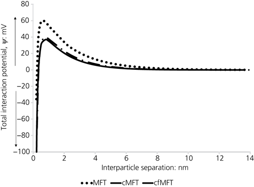
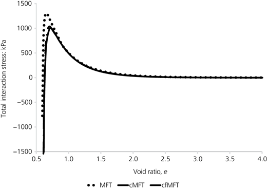
When the interparticle distance is converted to a void ratio and the potential function is converted to a stress function, the cfMFT sample with the highest hydrated specific surface area generates a marginally higher resistance to deformation at the closest approach of the particles (Figure 2). To convert the interparticle distance to void ratio (Equation 27), a monodispersed spherical particle with a radius R and close random packing (φ p) of 0.634 is assumed (Song et al., 2008)). Given that the particle volume (V p) rather than the effective particle volume is used in void ratio determination, R is the equivalent radius of a dehydrated particle.
V v is the volume of water around the particle and the non-interacting void spaces.
When Equation 19 is applied to determine the corresponding effective stress (σ′) from the known hydrostatic pressure, plots of the compressibility curves are shown in Figure 3 and compared with the compressibility measured using a large-strain consolidometer. Above approximately 5 kPa, the LLF model and LSC test are similar, but they deviate significantly at very low effective stresses where colloidal forces are more significant at the equilibrium average void ratio.
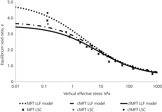
Compressibility curve derived from the LLF model (±6% relative uncertainty) compared with measured compressibility using a large-strain consolidometer
Compressibility curve derived from the LLF model (±6% relative uncertainty) compared with measured compressibility using a large-strain consolidometer
The compressibility function in Figure 3 derived from Equations 20–24 is adequately described using an LLF, and the associated parameters summarised in Table S2 in the online supplementary material.
Hydraulic conductivity function
Determination of the shape function (C e) in the modified Kozeny–Carman equation (Equation 7) is described in terms of a characteristic time factor in Equation 6. This makes the remaining unknown parameter the LLF rate function (n), which is determined using the centrifuge (Figure S2 in the online supplementary material). A summary of the material-dependent parameters in Equation 7 is provided in Table 3.
Material-dependent parameters in the modified Kozeny–Carman equation (Equation 7)
| e 0 (at time 0) | Characteristic particle size, L: nm | n (log-logistic rate) | |
|---|---|---|---|
| MFT | 4.395 | 10.2 | 1.0 |
| cMFT | 4.395 | 9.1 | 1.0 |
| cfMFT | 5.073 | 16.3 | 0.6 |
For non-interacting or weakly interacting particles undergoing settlement where the drainage tortuosity varies monotonically with the void ratio, n at infinite stresses approaches 1, thereby simplifying the permeability equation.
In flocculated slurries where the drainage tortuosity during settlement may vary from inter-floc aggregates at low effective stresses to intra-floc aggregates at high effective stresses, n is found at a plateau below 1. This effect is described in Figure S2 in the online supplementary material for MFT and cMFT (weakly interacting) and cfMFT (strongly flocculated). The settlement profiles from each of the centrifuge tests were fitted to an LLF to extract n, the equilibrium void ratio (e ∞) and t 50. The rate parameter in the cfMFT deposit follows a log-normal function given the larger influence of the sedimentation phase on the equilibrium void ratio at very low effective stresses. For the MFT and cMFT deposits, an exponential decay fit is used to estimate the equilibrium rate parameter as the effective stress goes to infinity. It is also observed that within the range of effective stresses measured with a centrifuge in Figure S2 in the online supplementary material, the equilibrium void ratio–average effective stress relationship closely follows the compressibility function described in Figure 3.
In practical applications where flocculated aggregate structures dominate the early settlement or sedimentation phase, n could be parameterised in terms of process variables (mineral surface area, flocculant type and dosages, flocculation efficiencies and transport energy dissipation rates). This may enable a feedforward approach to predicting the deposit deformation rate over time without the need for deposit sample testing using a centrifuge.
Figure 4 shows the variation of the shape parameter (C e) with the void ratio. C e parameterises the drainage path at different void ratios with a centroid at 50% of the total deformation (t 50). At high void ratios, the aggregate size of the flocculated slurry (cfMFT) drives the shape parameter.
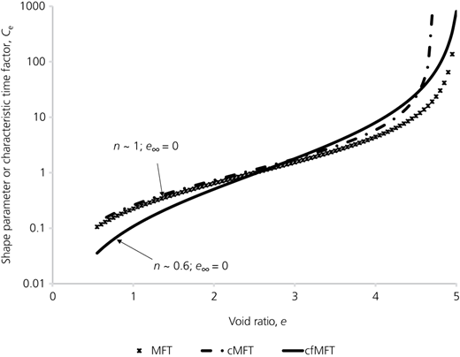
Variation of the shape parameter C e (dimensionless characteristic time) with the void ratio for MFT, cMFT and cfMFT deposits
Variation of the shape parameter C e (dimensionless characteristic time) with the void ratio for MFT, cMFT and cfMFT deposits
As settlement progresses and the void ratio decreases, steric forces limit the intra-aggregate drainage. In the flocculated slurry, steric forces due to the charged flocculant is responsible for the lower C e past the t 50, when compared to the non-flocculated MFT and cMFT slurries. Applying Equation 7 and the shape parameter in Figure 4, the hydraulic conductivity variation with void ratio is shown in Figure 5 and compared with those measured using a large-strain consolidometer.
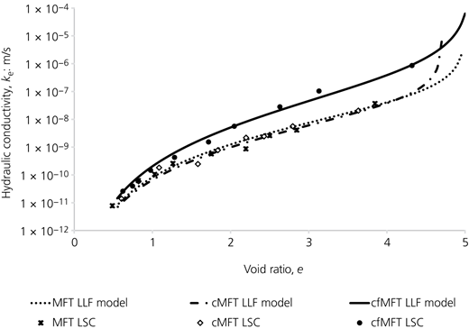
Hydraulic conductivity curve derived from the LLF model (±5.3% relative uncertainty) compared with LSC measurements
Hydraulic conductivity curve derived from the LLF model (±5.3% relative uncertainty) compared with LSC measurements
Settlement function
With the compressibility and hydraulic conductivity parameters determined, the finite-strain equation (Equation 1) could now be solved to determine the deformation rate. Two key assumptions in the finite-strain equation are that the solid fabric is incompressible under self-weight and the hydraulic conductivity is a function only of the void ratio (Gibson et al., 1981). However, polymeric flocculants are compressible, and so are, to a small extent, the precipitated hydroxide from the coagulant as they nucleate and grow during treatment and after deposition. Since the hydraulic conductivity is a function of the interparticle interaction, k(e) in Equation 1 would also be a function of the rate parameter n:
In differential form, Equation 28 could be written as
e ∞ is the equilibrium void ratio at a given effective stress, and recalling the boundary condition in the hydraulic conductivity shape function equation, the void ratio approaches 0 at infinite stress.
β is a material constant that is directly related to the compressibility of the coagulant and flocculant as they transition from a liquid phase at deposition to a solid as the void ratio approaches zero. β is approximated by the relationship
ρ L is the density of the compressible component in the liquid phase. β = 1 for MFT where no compressible phases are present and ∼4 and 20 for cMFT and cfMFT, respectively ( immediately after deposition is determined from the monodispersed spherical size in Table S1 in the online supplementary material, and is taken as the monodispersed spherical size of the dehydrated solid, which is equivalent to the starting mineral phase).
Using Equations 29–31, the deformation rate in the finite-strain equation could be modified as follows:
A reasonable settlement trajectory comparable with the observation is obtained when Equation 32 is solved for MFT, cMFT and cfMFT deposits placed in geocolumns (Figure 6).
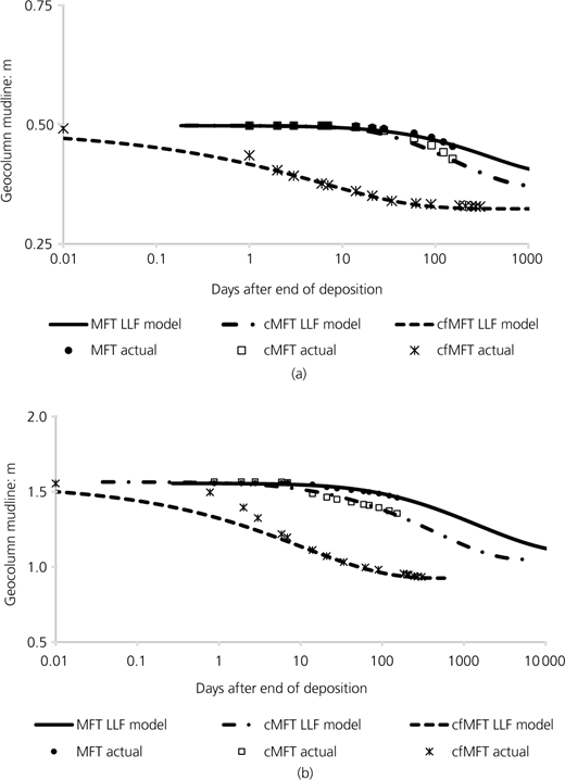
Measured mudline profiles for (a) 0.5 and (b) 1.5 m deposits of MFT, cMFT and cfMFT and mudline prediction using the LLF model (±6% relative uncertainty)
Measured mudline profiles for (a) 0.5 and (b) 1.5 m deposits of MFT, cMFT and cfMFT and mudline prediction using the LLF model (±6% relative uncertainty)
A deviation is noted for the cfMFT columns within the first week after deposition and the deviation increases with deposit height. It is likely that the assumption of monodispersed spheres that are non-segregating is a major driver, as larger floc sizes would be expected to settle much more quickly after deposition.
Comparison of models
A common approach to modelling the consolidation and settlement behaviour of fine tailings entails expressing the compressibility and hydraulic conductivity derived from the LSC test as power functions (Equations 33 and 34, respectively). The parameters A and B were obtained by fitting Equation 33 to the compressibility curve (e against σ′) from the LSC test and parameters C and D from the hydraulic conductivity curve (k against e). The power function parameters (Table 4) are the material properties input into the FSCA software, which implements a modified Equation 1 to determine the deformation rate.
Comparison of settlement profiles
Using the geocolumns as baseline, the settlement profiles obtained for MFT, cMFT and cfMFT using the LLF model and the LSC–FSCA model are shown in Figure S3 in the online supplementary material.
The settlement rate in the MFT deposit without treatment additives is quite slow, so the long-term predictions of the two models cannot be verified. However, the LSC–FSCA model overestimates the short-term settlement rate. The overestimation of the FSCA prediction is most likely due to a lack of creep correction of the LSC data. The FSCA software includes a creep function, which was not used in this set of analysis.
With coagulant addition (cMFT), the initial settlement rate is quicker than that of MFT, and while the LSC–FSCA model overestimates the early settlement rate at a low vertical stress in the 0.5 m geocolumn, it underestimates the initial settlement rate at a higher vertical stress in the 1.5 m geocolumn. The LLF model describes the initial settlement rates reasonably well for both the untreated MFT and the cMFT.
The initial settlement rate of the coagulated and flocculated deposit (cfMFT) is very high (the primary reason for adding a flocculant). The LLF model overestimates the initial settlement rate significantly within the first week in the 0.5, 1.5 and 5.0 m geocolumns (Figure S4 in the online supplementary material), beyond which the prediction describes the settlement profiles fairly well. The LSC–FSCA model underestimates the settlement rate in the 0.5, 1.5 and 5.0 m columns (for up to 2 years in the 5.0 m geocolumn). It is likely that the assumption of monodispersed spherical particles in the LLF model without allowance for a size distribution is responsible for the LLF model overestimating the initial settlement rate. Flocs with larger sizes would settle more quickly, leaving behind smaller flocs to define the mudline profile.
Comparison of deposit profiles
The deposit void ratio profiles calculated from density measurements at selected intervals (1, 3, 6 and 9 months) are shown in Figure 7. The LLF model significant underestimation of the density in the lower half of the 5 m geocolumn (at 1 month) reflects possible floc size segregation within the first week of settlement, which the LLF model does not attempt to describe. Beyond the first month, the LLF model describes the density profile reasonably well, except for the kink at the bottom 0.75 cm of the deposit at the 6- to 9-month mark resulting in an apparent reduction in the deformation rate. The cause of the kink is unclear; however, the location is adjacent to a sampling port where samples are taken periodically. The density profiles calculated using the LSC–FSCA model are significantly underestimated. Although the LLF model provides a better description of the density profile, neither model explains the full range of the deposit behaviour over time. This is most likely a consequence of the deposit segregation within the first few minutes of deposition, induced by the distribution of floc sizes in the slurry. The LSC test essentially ignores this initial settlement phase for the LSC–FSCA model, and the LLF model assumes a non-segregating monodispersed particle size.
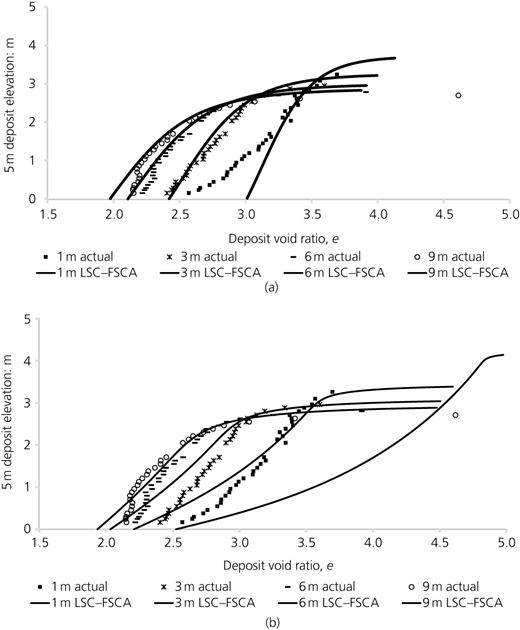
Void ratio deposit profiles from density measurements in a 5 m cfMFT geocolumn and profiles calculated from (a) the LLF model (±6% relative uncertainty) and (b) the LSC–FSCA model
Void ratio deposit profiles from density measurements in a 5 m cfMFT geocolumn and profiles calculated from (a) the LLF model (±6% relative uncertainty) and (b) the LSC–FSCA model
Conclusions
In pit lakes containing fluid tailings where the imposed vertical stress is primarily from self-weight, the LLF model provides a means for rapid prediction of the settlement profile during the deposition period to the end of consolidation.
The LLF model is a modification of Gibson’s finite-strain equation for reflecting interactions at the clay–water interface and the dependence of hydraulic conductivity on the solid fabric compressibility in cases where treatment additives induce a phase transformation between deposition and end of settlement. The LLF model is enabled by the assumption that the settlement profile of fine tailings follows an LLF where the total settlement parameter obtained from the LLF accounts for sedimentation, primary consolidation and creep phases.
The primary drawback of the LLF model is the need for material properties that are often difficult to measure accurately. While the specific hydrated surface area of the mineral phase can be measured by established methods such as methylene blue adsorption or use of ethylene glycol monoethyl ether, hydrated surface area measurement for the flocculant and the precipitated phases from coagulant addition is not standard. Nevertheless, techniques such as water (H2O) Brunauer–Emmett–Teller analysis could be used in particular for non-ionic flocculants. The Hamaker constants are also better measured for each of the components. However, this may be difficult in real deposits, as the surface characteristics of the mineral components in the deposit may differ from those of pure minerals used to determine the Hamaker constants.
Acknowledgements
The author would like to thank the tailings staff at Coanda Research and Development for preparing the MFT, cMFT and cfMFT samples; conducting the LSC tests; monitoring the geocolumns; and providing valuable suggestions to improve the paper.
